By Jay Parmar
This article on Jupyter Notebooks(previously known as IPython Notebooks), does not require any pre-requisite knowledge and does not assume any familiarity with the framework. This blog is an introductory article where I will primarily address the following questions:
- What is Jupyter Notebook?
- How to install the Jupyter Notebook environment?
- How to run or open Jupyter Notebook?
- What are the different components of Jupyter Notebook?
- What are cells in a Jupyter Notebook?
- How to write in Markdown language?
- What are the magic commands in Jupyter Notebook?
- How to download and share Jupyter Notebook?
After reading this blog, you will be able to:
- Install the Jupyter Notebook environment
- Open Jupyter Notebook
- Understand various components
- Download and share Juypter Notebooks
Along with the above questions, you will also learn writing in Markdown language in Jupyter notebooks. Let's get started with the first question.
What is Jupyter Notebook?
If you are a student, you must be using a class notebook to take various class notes, or if you are a business professional, you might be using a writing pad to pen down important notes, either for your purpose or to present to someone else.
The typical content that goes in a student's notebook can be text in various formats such as bold and italic, or a table, a mathematical equation, or creative stuff like hand-drawn images and so on. Not to forget that if it's a programmer's notebook, it will also contain a lot of programming code.
Now, you want to continue with this practice of writing all such stuff in a single place online. Jupyter notebook comes to the rescue here. It is a web-based platform that allows you to write narrative text in various formats, include a table or an image, write equations and code in various programming languages, all in one place.
Apart from this, Jupyter notebook also allows you to write LaTeX code, include HTML code and embed a YouTube video. I will talk about how to do so in a bit, but first let's see what its official documentation says:
The Jupyter Notebook is an open-source web application that allows you to create and share documents that contain live code, equations, visualizations and narrative text. Uses include data cleaning and transformation, numerical simulation, statistical modelling, data visualization, machine learning, and much more.
To get a look and wheel of what a Jupyter Notebook looks like, be sure to catch the following video by Quantra which provides a short yet descriptive explanation about it:
You can also refer to the below-given list to get an intuitive idea about how a Jupyter notebook looks like:
A backdrop: The Jupyter Notebook is one of two facets of the Jupyter project which started to develop open-source, open-standards for interactive computing across dozens of programming languages. Another being JupyterLab which is the advanced version of Jupyter Notebook interface. However, both operate in a similar fashion.
Now that you have an idea about what Jupyter notebooks are, let's see its installation process.
How to install Jupyter environment?
jupyter notebook
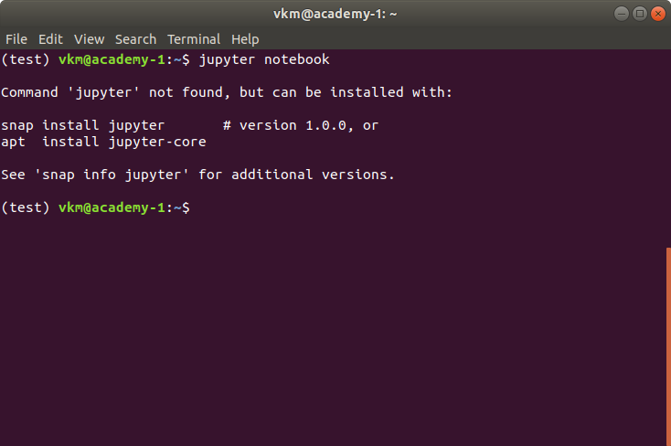
If the above command fails, you can continue reading this section. Otherwise, you can safely skip this and proceed to the next section. In case the command fails and you get the error similar (not exact) to the one shown below, continue with this section to understand the installation process.
Two popular methods using which Python can be installed on your workstation. They are
- Installing Python using Anaconda Distribution
- Installing Raw Python
While Jupyter runs code in many programming languages, Python is a requirement for installing the Jupyter Notebook.
Installing Jupyter Notebook using Anaconda
If you have installed Python using Anaconda Distribution, you are good to go. Anaconda Distribution includes Python, the Jupyter Notebook, and other commonly used packages for the scientific community.
If you don't have any version of Python installed, the recommended way to install Python is using Anaconda Distribution. It should be pretty simple to get Python installed.
- First, download the latest version of Anaconda Distribution.
- Second, install the downloaded version of Anaconda.
Bam! You have installed Jupyter Notebook. To check whether the installation is successful or not, and run the Jupyter Notebook, run the following command in the Anaconda prompt or command prompt (Windows) or terminal (Mac/Linux).
jupyter notebook
If you get an error upon running the above command (which should not happen), try the following method.
Installing Jupyter Notebook using pip
When you install Python directly from its official website, it does not include Jupyter Notebook in its standard library. In this case, you need to install Jupyter Notebook using the pip. The process is as follows:
- Open a new command prompt (Windows) or terminal (Mac/Linux)
- Execute the following command to install Jupyter Notebook
python -m pip install jupyter
or if you are using Python 3
python3 -m pip install jupyter
or simply
pip install jupyter
Congratulations, you have installed Jupyter Notebook! Onward to running it.
How to run or open Jupyter Notebooks?
After you have installed the Jupyter Notebook on your computer, you are ready to run the notebook server.
If you are reading this article from the beginning, then you might already know how to run Jupyter Notebook. However, if you have skipped the previous sections and directly jumped here, the below mentioned steps shows how to run the Jupyter Notebook.
First, open a new command prompt (Windows) or terminal (Mac/Linux) on your workstation, and second, execute the following command:
jupyter notebook
Upon executing the above command, the terminal or command prompt will print some information about the Jupyter Notebooks being loaded. It might look something like as shown in the below snapshot. Be mindful that the information printed would be different for each workstation.

Keep the terminal open as it is. It will then open the default web browser with the URL mentioned in the command prompt or terminal.
When the notebook opens in your browser, you will see the Notebook Homepage as shown in the below snapshot. This will list the notebook files and subdirectories in the directory where the notebook server was started.

In case you are using Anaconda distribution for Python, you can open Anaconda Navigator (using the Start Menu(Windows), Applications folder(Mac), or Softwares folder(Linux)) shown below which allows you to open Jupyter Notebook using point and click.

Once the Navigator application is open, you can click on the Launch button within the Notebook dialogue to launch the Jupyter Notebook application. Upon clicking the Launch button, you will be presented by the homepage that we'd seen earlier.
Now, let's understand how Jupyter environment works, I won't be going technical, though. As the Jupyter Notebook is a web application, it works on a server-client architecture. When you execute the command jupyter notebook, the Jupyter software starts the server locally in the console where the command is executed, and the Jupyter Notebook homepage that opens in the web browser works as the client. Whatever you perform, that is, create or upload a new notebook, or save the existing one, the client notebook on which you are working, will keep communicating with the server running in the console/command line.
To keep notebooks running smoothly, we need to keep the command prompt or terminal open, even after it has opened homepage. If you close it, notebooks that you are working with, won't be able to communicate with the local server, and hence, any work you do, will not be saved on persistent memory.
The next step is to learn various components of Jupyter software.
What are the different components of Jupyter notebooks?
I assume that you are following the chronological order of this article. If so, then you have learned what Jupyter notebooks are, how to install it, and how to run and open it. If not, then I would recommend you to go through them to get an overall picture. Nevertheless, if you are already familiar with those parts, go on and keep learning.
In this section, I will explain the various components of Jupyter software. When you start Jupyter Notebook application, and you'll be presented with the homepage. Let's start exploring it. Below shown is the snapshot of the homepage that you'd seen earlier, but with numbers assigned to each component to make our learning easier.

Here's the description of each numbered point shown in the snapshot.
- It is the URL on which Jupyter server is running. If you are running the Jupyter on localhost, this would be the same URL shown in the console when you started Jupyter software.
- The Files tab lists the directories and files in the home folder, which usually is the home directory of the user logged in to the computer.
- The Running tab shows you a list of all open notebooks. When you start a new notebook or open an existing notebook, a kernel will get attached to it. All such running kernels will be listed under this tab.
- If you want to open an existing Jupyter notebook(that ends with .ipynb extension), it needs to be listed in the Files tab. If it is not listed, you need to upload it using the Upload button which will open a file browser for you to load the file.
- Quit and Logout buttons allow you to logout and shutdown the server. When you quit, all the opened notebooks will be closed, and the server will get shutdown.
- The New button allows you to create a new notebook, text file, folder, or terminal. The snapshot shown below shows that you can create a notebook in Python, Julia, and R language. The notebook that you create will be associated with a respective kernel. When you install Jupyter environment as shown in the previous section, it is very likely that you will have only one option for the kernel, that is, Python. In order to add new languages, you can refer to this link.

You can create a new notebook by clicking on the respective language name. Regardless of what language you choose, the new notebook that you create will have the same appearance. The difference would be in terms of the kernel attached to it. If I click on Python 3 on the dropdown opened, a new notebook with Python kernel attached to it will be created. The empty Jupyter notebook is shown in the snapshot below. (Obviously without numbers :p)

The newly created notebook has various components which are explained below:
- The title is the name of the notebook. The title you set becomes the file name for the notebook, and it will have the extension as .ipynb which stands for IPython NoteBook.
- The checkpoint shows you the time when your notebook was saved last.
- The menu bar lists various menus that allow you to download the notebook(in multiple formats), open a new notebook, edit the notebook, customise the headers, manipulate cells, nudge the kernel, access help and so on.
- The shortcut bar lists commonly used shortcuts such as save to save the notebook, add a cell, cut, copy to manipulate cells, up and down to navigate between cells, run to execute the cell, and so on. Any extension that you add to Jupyter will have its shortcut on this bar. We will learn what extensions are in the latter part of this article.
- The Kernel shows you the current kernel associated with the notebook. In our case, the kernel is Python 3. The circle beside the kernel shows the status of the kernel. The hollow circle represents that it is ready to take input and run a cell. When a kernel is executing code or processing anything, it changes to solid.
- A cell is the part of a notebook where all the magic happens. Cells are explained in detail in the following section.
What are cells in a Jupyter Notebook?
Any text or code that you write goes in the cell. Cells are the building block of any Jupyter notebook. Cells operate in two modes: command and edit mode, and they are of mainly three types: code, markdown, and Raw NBConvert.
The command mode allows you to manipulate cells. That is, the action you perform has to do with the cell as a whole. The command mode is represented by a grey border around the cell with a blue indication, as shown in the below snapshot.

Some of the operations (along with their shortcuts) that you can perform when a cell is in the command mode are as follows:
- Insert a new cell -- Key in
Ato insert a new cell above, andBto insert a new cell below the current cell.- When a new cell is inserted, it will be a code type cell, by default. We will look at various types in a while.
- Merge existing cells --
Shift-Mallows to merge selected cells or to merge the current cell with the cell below the current cell. - Copy cells --
Ccopies selected cells. - Cut cells --
Xcuts selected cells. - Paste cells -- Use
Shift-Vto paste cells. - Delete existing dells -- Pressing
D,Ddeletes the current cell. Be careful with this shortcut. - Change the type of a cell -- The shortcut
Ychanges the cell type to code,Mchanges the cell type to markdown, andRchanges the cell type to raw. - Convert the cell to a heading -- There are six heading types in a Jupyter notebook. This works with markdown cell type only. Heading 1 is the largest heading and heading 6 is the smallest heading.
1,2,3,4,5, and6are used to change the cell type to the respective heading size. - Find and Replace in existing cells -- Pressing
Fopens find and replace dialogue box. - Save and mark the Checkpoint of the notebook -- Use
Shift-Sto save the notebook. - Toggle line numbers in a cell -- Pressing
Ltoggles line number in the current cell. - Toggle the output of a cell --
Oallows you to toggle the output of the current cell. - Interrupt the kernel -- Keying
I,Iinterrupts the kernel. That is, if any process is being executed by the kernel gets stopped. - Scroll the notebook --
Spacescrolls the notebook down,Shift-Spacescrolls the notebook up. - Enter the edit mode -- Pressing
returnkey changes the mode of a cell to the edit mode.
The shortcuts mentioned above work only in the command mode cells. Another mode that a Jupyter notebook cell supports is the edit mode. This mode specifically allows you to edit the content of a cell and work with it. You can enter into the edit mode of a cell by pressing the return key or by a mouse click inside a cell. The border around cell changes to Green when the cell is in the edit mode, as shown in the below snapshot.

Once the cell is in edit mode, you can start writing code or text. The below-mentioned are some of the operations that you can perform while the cell is in the edit mode.
- Auto-Completion of code -- Use
Tabkey to use this facility. It works only for code type cells. In markdown cells, it will simply put tab spaces. - Indentation of code -- Jupyter notebooks inherently perform indentation whenever required. However, if you want to change indentation manually, use
Ctrl-]to indent the code in code type cells. In markdown cells, it will insert spaces according to the specifications of the tab key. - Dedentation of code -- Anytime you want to dedent the code, use
Ctrl-[to do so. In markdown cells, this shortcut works similar toShift-Taband dedents the content. - Commenting a code -- Use
Ctrl-/to comment a code. In markdown cells, this shortcut does not have any effect. - Execute of a cell -- Once you write code or text in the cell, you need to execute it to process the content written by you. There are three primary ways to do so.
- Run the current cell and select the next cell - Use
Shift-Enterto perform this action. - Run selected cells - Use
Ctrl-Enterto run selected cells or the current cell. - Run the current cell and insert a new cell - Press
Alt-Enterto execute the current cell and insert the new cell below the current cell.
- Run the current cell and select the next cell - Use
- Split a cell -- Use the shortcut
Ctrl-Shift-Minusto split the current cell into two separate cells at the cursor. - Entering a Command Mode -- Use
Ctrl-Mor pressEsckey to exit from the edit mode and enter into the command mode.
By now, you have already encountered code and markdown cell types quite a few times. In case you are not aware of the two, now is the time where I will explain them in detail. I will restrict the discussion for these two types only; I won't be covering the Raw NBConvert type in this article.
Jupyter notebook cells can be multiple types. Often used types are code and markdown. The code type cells allow you to write live programming code. That is, you can perform any sort of programming in them. Once you run or execute a code cell, Jupyter notebook will present the output just below the cell. This is shown in the below snapshot.

In contrast, whatever written in the markdown cell, will get printed in the cell itself, as shown below:

There are two cells in the above snapshot. The first cell numbered four, is the code cell, which allows tying in Python code as we are working with Python kernel notebook. The next cell is the markdown cell where the normal text is written.
As can be seen, code cells have a number associated with them, whereas markdown cells do not have any numbering. Numbering code cells helps in two ways: First, it shows the sequence in which code executed, and second, it allows us to differentiate between the code cells and markdown cells visually. Now that you know the basics of cells and their workings, let's see how you can use markdown.
How to write down in Markdown in Jupyter Notebook?
It is the markdown functionality that brings interactivity to Jupyter environment. Markdown cells not only lets you write text, but it allows you to format it, add a hyperlink, and include HTML code. Additionally, it also allows you to define ordered and unordered lists, insert images and tables, add mathematical equations, write in LaTex, and so on. It even allows you to write programming code within the text without losing any syntax.
Once you have a markdown cell (you can use the shortcut M in command mode to convert a code cell to markdown cell), you can start writing the text the way you want. Below-mentioned are the functionalities supported by markdown cells.
Headings
To create headings, use the hash symbol # followed by a space and the heading. Doing so creates a title or level 1 heading. If you want to create a sub-heading, use ## followed by a space and the sub-heading. The notebook allows creating headings up to six levels. Each level will have the equivalent number of # marks, as shown below:
# Heading 1 - Title ## Heading 2 - Heading ### Heading 3 - Sub-heading #### Heading 4 - Heading at level four ##### Heading 5 - Heading at level five ###### Heading 6 - Heading at level six
Emphasis
You can make text italic by surrounding it with * or _.
| Input | Output |
|---|---|
*This is italic text.* |
This is italic text. |
_This is italic text._ |
This is italic text. |
You can make text bold by surrounding it with ** or __.
| Input | Output |
|---|---|
**This is italic text.** |
This is italic text. |
__This is italic text.__ |
This is italic text. |
Monospace Fonts
If you want to refer to some code, filename, or file path within the text, you can use monospace fonts to differentiate the normal text and the monospace fonts. You can do so by surrounding the text with a single back quotation mark. (`)
This is written in monospace fonts.
Line Breaks
You can use the HTML line break tag <br> to insert the carriage-return within a line to break it.
Font Color
You can change the color of text by using the HTML font tag along with its color attribute. For example, to color the text in blue, you can use the following code:
<font color='blue'>The color of this text is blue.</font>
The output of the above code is shown below:
The color of this text is blue.
Change the color attribute of the font tag to change the text color. Remember, not all markdown text works with the font tag. Hence, review it carefully.
Blockquotes
Use a greater than sign > followed by a space to type or insert a blockquote. The output will be indented with Grey horizontal line to the left of it. For example, the output of the line > Jupyter makes life easy! will be as follows:
Jupyter makes life easy!
Unordered Lists
You can create an unordered list using the minus or dash sign - followed by an item name. The next time goes on the next line.
- Item 1 - Item 2 - Item 3
To create a sub list, the same procedure is followed; however, with an indentation. Can you create a list as shown below:
- Item 1
- Item 1.1
- Item 1.2
- Item 1.2.1
- Item 2
- Item 2.1
- Item 2.2
In Jupyter, the first-level list items would generally have solid circles, the next level would have solid squares and the subsequent levels would have hollow circles.
Ordered Lists
Ordered lists can be created by manually specifying the item number such as 1 followed by a dot and space, and finally, item name. To create a sub-list, the procedure would be the same.
- Chapter 1
- Section 1.1
- Chapter 2
- Section 2.1
- Section 2.2
Horizontal Lines
You can create a horizontal line by using three asterisks ***.
Hyperlinks
You can convert any normal text into a hyperlink by surrounding it with square brackets followed by the actual link in parenthesis. For example,
[QuantInsti's Blog](https://blog.quantinsti.
will result in
Images
The format to insert an image in a markdown cell is very similar to that of hyperlinks. Only the difference is that it prefixes ! before the content. First, the exclamation mark followed by the name of the image in square brackets, and finally URL in the parenthesis. This is shown below:

Geometric Shapes
A UTF-8 Geometric Shape can be included in a Jupyter notebook by using its decimal reference number. Use the following format to insert any of the shapes.
&#reference_number;
A black circle can be inserted, as shown below:
●
Programming Code
You can embed programming code within the text using triple backticks followed by programming language name and ending by triple backticks. Below is the example for Python code embedded within the text.
```python
def func(x):
 return x**2
```
Similarly, the programming code for another language can be written. For example, below code is for Javascript.
```javascript
console.log('Hello World!')
```
LaTeX Equations
By courtesy of MathJax, you can include mathematical expressions either inline or separately in markdown cells. To type inline, equations are surrounded by $. To print equations separately on a new line, they are surrounded by $$. For example, the formula to calculate the mean value can be written as
$$\mu = \frac{1}{n}\sum_{i=1}^{n} x_i $$
which results in the following:

Inline equations can be written as $x_t = \phi x_{t-1} + \epsilon_t$ which results in

You can refer to this thread which lists various LaTeX commands that can be used in markdown cells.
Tables
You can create tables in markdown cells, as shown below:
|This|is|
|-|-|
|a|table|
Columns are separated by vertical bar | and rows are written in a new line. The above table is generated, as shown below:
| This | is |
|---|---|
| a | table |
What are the magic commands in Jupyter Notebook?
Jupyter notebook software comes with a bunch of built-in commands which adds interactivity while working with it. They are called magic commands in Jupyter environment. These commands are dependent on the interpreter or kernel with which you are working. To see which magic commands are available, you can run the following magic command in the code cell:
%lsmagic
These magic commands are prefixed with the % value. Following are some of the commonly used magic commands along with their functionality:
%autosavecommand autosaves your notebook periodically.# Save notebook every 60 seconds %autosave 60
%cdchanges the current working directory to the new directory given as an argument.%clearand%clscommand clear the output of the current cell.%envallows you to list all environment variables as well as set the value of particular environment variables.%historyshows the history of the previously executed magic commands.%history
%lslists the content of the current directory.%ls
%matplotliballows you to plot charts inline within a notebook.%matplotlib inline
%notebookcommand adds the interactivity while plotting charts.%pdballows you to debug the code. This magic command is the Jupyter version of Python debugger.%pipenables you to list and install all available packages from Jupyter environment.%pip install pandas
%wholist all variables from the global scope.stock = 'AAPL' price = 222.15 %who str
%loadinserts the code from an external script.%load ./hello_world.py
%runallows you to run Python code.%run ./sample_notebook.ipynb
%timedisplays the time taken by a cell for execution.
If you are using Anaconda Python, then magic commands mentioned above should work without any issue. Otherwise, you may require to install the following packages:
- ipython-sql
- cython
How to download and share Jupyter Notebook?
Being a programmer, you often want the work that you have done to be shared with other colleagues. Keeping this in mind, Jupyter environment allows you to download files in multiple formats such as HTML file(.html), LaTeX file(.tex), GitHub flavoured Markdown file(.md), PDF file(.pdf), reStructured file(.rst), and so on. The Download as option in the File menu allows you to download the notebook in a format of your choice, as shown below:

When you download a notebook, it will be downloaded in whatever state it is. That is the output of executed cells, any error that you might have as an output will be as it is. Hence, it is essential that you make a notebook ready to be shared. To do so, you can perform the following steps:
- Go to Cell menu, select All Output option, and finally choose the Clear option. This action will clear the output of all cells.
- Next, go to Kernel menu, and select the Restart & Run All option. This action will restart the kernel and execute all cells.
After performing the above steps, ensure that the notebook is in the state in which you would like to share with others.
Besides exporting notebooks to your local workstation, you can create, list and load it on GitHub Gists. Gists are a way to share your work on the cloud. You can find more information here.
Also, you can use JupyerHub, which serves Jupyter notebooks to multiple users. In other words, it is the hosting platform for notebooks on a server with multiple users.
Additionally, you can use the nbviewer to render Jupyter notebooks as static web pages. Platforms such as RISE and nbpresent allow you to convert Jupyter notebooks to slideshows.
Final Thoughts
I hope this introductory guide to Jupyter notebooks provides you with the foundation. In this relatively a multi-part article, First, I started with the explanation of Jupyter notebook, its installation process, running locally on your workstation and so on. Next, during the process, you also got exposed to various components of Jupyter notebooks and keyboard shortcuts. Then, you learnt writing in markdown language. After that, you learnt various magic commands in Jupyter notebook. Finally, you learnt how to download and share Jupyter notebooks.
Thanks for reading.
There are many people who might be new to Python or programming in general or never created any trading strategy. The learning curve could be steep if you are a beginner in both these skills. However, you can build the required skills gradually and practice regularly on the hands-on learning exercises given in our course by enrolling here: Algorithmic Trading for Everyone.
If you want to learn various aspects of Algorithmic trading then check out our Executive Programme in Algorithmic Trading (EPAT®). The course covers training modules like Statistics & Econometrics, Financial Computing & Technology, and Algorithmic & Quantitative Trading. EPAT® is designed to equip you with the right skill sets to be a successful trader. Enroll now!
Disclaimer: All data and information provided in this article are for informational purposes only. QuantInsti® makes no representations as to accuracy, completeness, currentness, suitability, or validity of any information in this article and will not be liable for any errors, omissions, or delays in this information or any losses, injuries, or damages arising from its display or use. All information is provided on an as-is basis.