
In the previous blog, we have learnt how to perform the forward propagation. In this blog, we will continue the same example and rectify the errors in prediction using the back-propagation technique.
What is Back Propagation?
Recall that we created a 3-layer (2 train, 2 hidden, and 2 output) network. But once we added the bias terms to our network, our network took the following shape.
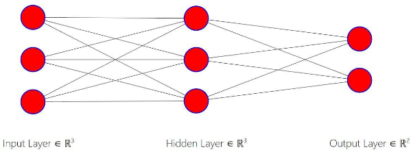
After completing forward propagation, we saw that our model was incorrect, in that it assigned a greater probability to Class 0 than Class 1. Now, we will correct this using backpropagation.
Why Backpropagation?
During forward propagation, we initialized the weights randomly. Therein lies the issue with our model. Given that we randomly initialized our weights, the probabilities we get as output are also random. Thus, we must have some means of making our weights more accurate so that our output will be more accurate. We adjust these random weights using the backpropagation.
Loss Function
While performing the back-propagation we need to compute how good our predictions are. To do this, we use the concept of Loss/Cost function. The Loss function is the difference between our predicted and actual values. We create a Loss function to find the minima of that function to optimize our model and improve our prediction’s accuracy. In this document, we will discuss one such technique called Gradient Descent which is used to reduce this Loss. Depending on the problem we choose a certain type of loss function. In this example, we will use the Mean Squared Error or MSE method to calculate the Loss. In the MSE method, the Loss is calculated as the sum of the squares of the differences between actual and predicted values.
Loss = Sum (Predicted - Actual)²
Let us say that our Loss or error in prediction looks like this:
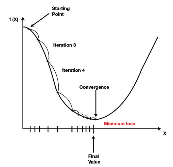
We aim to reduce the loss by changing the weights such that the loss converges to the lowest possible value. We try to reduce the loss in a controlled way, by taking small steps towards the minimum loss. This process is called Gradient Descent (GD). While performing GD, we need to know the direction in which the weights should move. In other words, we need to decide whether to increase to decrease the weights. To know this direction, we must take the derivative of our Loss function. This gives us the direction of the change of our function. Below is an equation that shows how to update weights using the Gradient Descent.
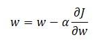
Here the alpha term, α, is known as the learning rate and is multiplied by the derivative of our Loss function (J) (Please recollect that we have discussed how to calculate the derivatives of a function in the chain rule of derivatives document). We subtract this product from our initial weight to update it. It is also to be noted that this form of the derivative is known as the partial derivative. While finding the partial derivative, the remaining terms are treated as constants.
If you consider the curve in the above figure as our loss function with respect a feature, then we can say that the derivative is the slope of our loss function and represents the instantaneous rate of change of y with respect to x. While performing back-propagation we are to find the derivative of our Loss function with respect to our weights. In other words, we are asking “How does our Loss function change when we change our weights by one unit?”. We then multiply this by the learning rate, alpha. The learning rate controls the step-size of the movement towards the minima. Intuitively, if we have a large learning rate we are going to take big steps. In contrast, if we have a small learning rate, we are going to take small steps. Thus, the learning rate multiplied by the derivative can be thought of as steps being taken over the domain of our Loss function. Once we make this step, we update our weights. And this process is repeated for each feature.
In the example below, we will demonstrate the process of backpropagation in a stepwise manner.
Backpropagation Stepwise
Let’s break the process of backpropagation down into actionable steps.
- Calculate Loss Function; (i.e. Total Error of Neural Network)
- Calculate the Partial Derivatives of Total Error/Loss Function w.r.t. Each Weight
- Perform Gradient Descent and Update Our Weights
The first thing that we need to do is to calculate our error. We define our error using MSE formula as follows:
Error = (Target - Output) ²
This is the error for a single class. If we want to compute the error in predicted probabilities for both the classes of an example. Then we combine errors as follows.
Total Error = Error₁ + Error₂
Where Error₁ and Error₂ represent the errors in predictions for the two classes. Recall that our output was a3 which was computed to be:
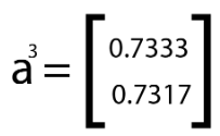
denoting a lesser prediction for Class 1 than Class 0. In our example, we stated that Class 1 should have had a greater probability and thus been our predicted class label. To further illustrate this, we create some hypothetical target probability values for Class 0 and Class 1 for the ease of understanding.
Let us assign the following target values(t) for output layer probabilities:
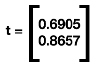
Now, let’s compute the errors.
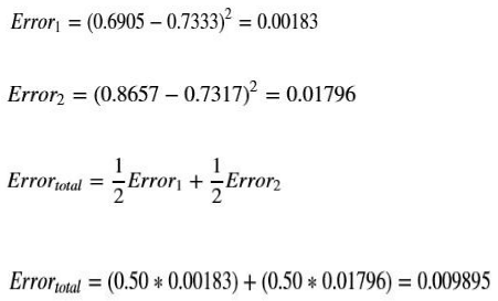
So, the Total Error in the prediction is 0.009895.
Each error contains the predicted value, and each predicted value is a function of the weights and inputs from the previous layer. Extending this logic, one can say that our total error is a function of the different weights or in other words is multivariate. And because we have multiple weights, we must use partial derivatives, or find out how a change in one specific weight changes our total error equation. This means that we must use the chain rule to decompose the errors.
Once we have computed the partial derivative of our error function with respect to a weight, we can then apply Gradient Descent equation to update the weights. We repeat this for each of the weights and for all the examples in the train data. This process is repeated many times and every such pass over all the examples is called an Epoch. We perform these passes until there is a convergence in the loss, or the loss function stops improving.
Now that we have understood the process of backpropagation, let’s implement it. To perform the backpropagation, we need to find the partial derivatives of our error function w.r.t each of our weights. Recall that we have a total of eight weights (i.e. Before adding bias terms). We have two weights from our first input to our hidden layer and two weights from our second input to our hidden layer. We also have four weights from our hidden layer to our output layer. Let’s label these weights as follows.
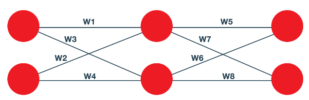
We call the weights from our first input neuron as w1 and w3, and the weights from the second input neuron a w2 and w4. The weights from our hidden layer’s first neuron are w5 and w7 and the weights from the second neuron in the hidden layer are w6 and w8. In this example, we will demonstrate the backpropagation for the weight w5. Note that we can use the same process to update all the other weights in the network.
Let us see how to represent the partial derivative of the loss with respect to the weight w5, using the chain rule.
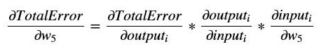
Where 'i' in the subscript denotes the first neuron in the output layer. To compute the first derivative of the chain, we express our total error equation as:

Here j in the subscript denotes the second neuron in the output layer. The partial derivative of our error equation with respect to the output is:
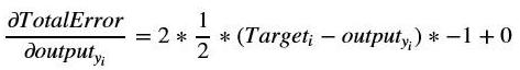
Substituting the corresponding values, we will get:
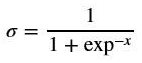
Next, we find the second term in our equation. Recall that in the forward propagation step, we used the sigmoid or logistic function as our activation function. So, for calculating the second element in the chain we must take the partial derivative of the sigmoid with respect to its input.
Now, recollect that the sigmoid function is as follows:
The derivative of this activation function can also be written as follows:
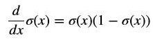
The derivative can be applied for the second term in the chain rule as follows:
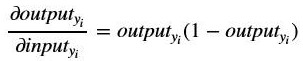
Substituting the output value in the equation above we get:
0.7333(1 - 0.733) = 0.1958
Next, we compute the final term in the chain equation. Our third term encompasses the inputs that we used to pass into our sigmoid activation function. Recall that during forward propagation, the outputs of the hidden layer are multiplied by the weights. These linear combinations are then passed into the activation function and the final output layer.
Recollect that these weights are given by Theta2.
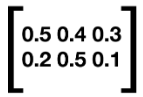
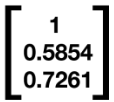
And let us say that the outputs from our Hidden Layer are given as follows.
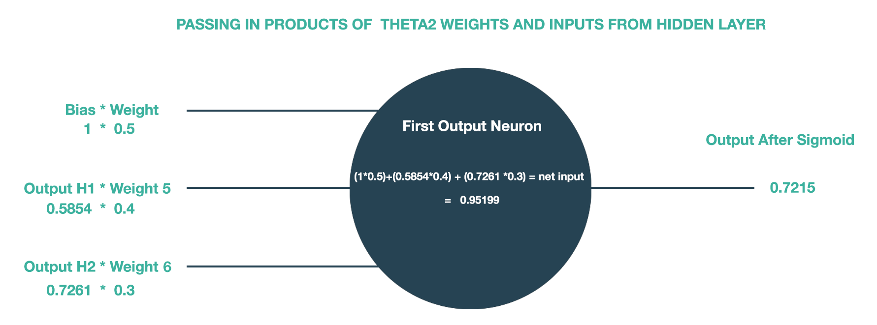
To visualize the matrix multiplication that follows, please see the diagram below:
Here, H1 and H2 denote the hidden layer neurons.
Our equation for the third term is concerned with the partial derivative of the input into the node with respect to our fifth weight. Our fifth weight is associated with the second neuron in our hidden layer as shown above. So, when we perform the partial differentiation with respect to w5, all the other weights are treated as constants and their derivatives are taken as zeros.
So, when the input which is the value we received from the combination of Theta 2 and the outputs of our Hidden Layer is differentiated, then the result looks like is:
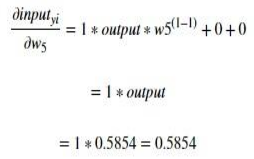
Where output is the Hidden neuron H1’s output.
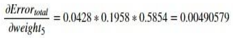
Now that we have found the value of the last term in our equation, we can compute the product of all three terms to derive the partial derivative of our error function w.r.t w5.
We can now use this partial derivative in our Gradient Descent equation as shown, to adjust the weight w5.
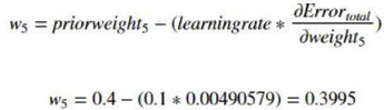
So, the updated weight w5 is 0.3995. As you can see, the value of w5 has changed little, as our learning rate (0.1) is very small. This small change in the value of w5 may not affect the final probability much. But, if the same process s performed multiple times for both the examples and the weights are adjusted for every run (epoch) then we will get a final neural network that has the expected prediction.
Updating our Model
After completing backpropagation and updating both the weight matrices across all the layers multiple times, we arrive at the following weight matrices corresponding to the minima.
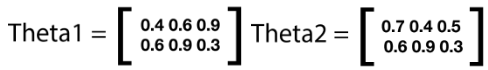
We can now use these weights and complete the forward propagation to arrive at the best possible outputs. Recall that the first step in this process is to multiply the weights with inputs as shown below.
![]()
Recall that we take the transpose of our X matrix to ensure that our weights line up. Here we are using our new updated weights for Theta1, and our matrix multiplication will now look like the following:
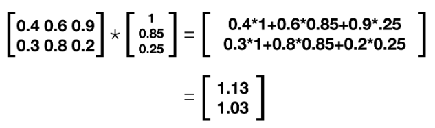
This is our new z² matrix, or the output of the first layer.
Recall that our next step in forward propagation was to apply the sigmoid function element-wise to our matrix. This will yield the following:
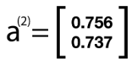
Here, a² is the output of the hidden layer. Again, this is our activation layer and will serve as the new input into our final layer. We again add back our bias term and thus our new a² looks like the following:
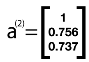
Now we will use our new values for our Theta2 weight matrix to create the input for our output layer. We now perform the following computation to arrive at the new value of our z3, or the output matrix.
![]()
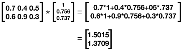
After this matrix multiplication, we apply our sigmoid function element-wise and arrive at the following for our final output matrix.
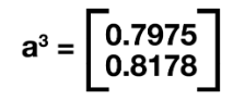
We can see here that after performing backpropagation and using Gradient Descent to update our weights at each layer we have a prediction of Class 1 which is consistent with our initial assumptions.
If you want to learn how to apply Neural Networks in trading, then please check our new course on Neural Networks In Trading.
