By Umesh Palai
In this article, we are going to develop a machine learning technique called Deep learning (Artificial Neural network) by using tensor flow and predicting stock price in python. At the end of this article you will learn how to build artificial neural network by using tensor flow and how to code a strategy using the predictions from the neural network. Once the strategy is coded from the neural network's predictions, python backtesting is the essential next step to verify whether those predictions actually produce profitable trades, the Quantra course on Backtesting Trading Strategies covers exactly this validation process.
System Requirements: Python 3.6
If you are new to Neural Networks and would like to gain an understanding of their working, I would recommend you to go through the following blogs before building a neural network.
Working of neural networks for stock price prediction
Training neural networks for stock price prediction
Coding The Strategy
Importing Libraries
We will start by importing all libraries. Please note if the below library not installed yet you need to install 1st in anaconda prompt before importing.
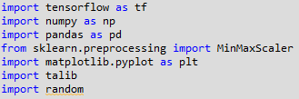
TensorFlow is an open-source software library for dataflow programming across a range of tasks. It is a symbolic math library, and is used for machine learning applications such as deep learning neural networks. Wikipedia.
Refer to this article to get detailed steps on installing TensorFlow GPU .
Numpy is a fundamental package for scientific computing, we will be using this library for computations on our dataset. The library is imported using the alias np.
Pandas will help us in using the powerful dataframe object, which will be used throughout the code for building the artificial neural network in Python.
Scikit-learn is a free software machine learning library for the Python programming language. It features various classification, regression and clustering algorithms including support vector machines. Wikipedia
Matplotlib is a Python 2D plotting library which produces publication quality figures in a variety of hardcopy formats and interactive environments across platforms
TA-Lib is a technical analysis library, which will be used to compute the RSI and Williams %R. These will be used as features for training our artificial neural network. We could add more features using this library. Develop your skills and learn about more applications and practices of neural network in trading with an advanced course.
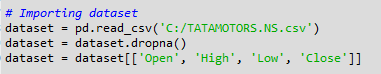
Importing the dataset
We are going to use daily OHLC data for the stock of Tata Motors trading on NSE for the time period from 1st January 2000 to 30 Aug 2018. We 1st import our dataset .CSV file named ‘TATAMOTORS.NS.csv’ saved in personal drive in your computer. This is done using the pandas library, and the data is stored in a dataframe named dataset. We then drop the missing values in the dataset using the dropna() function. We choose only the OHLC data from this dataset, which would also contain the Date, Adjusted Close and Volume data. We will be building our input features by using only the OHLC values.
Please note you can also download these data from my github.
Preparing the dataset
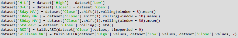
We then prepare the various input features which will be used by the artificial neural network to train itself for making the predictions. Please note I have limited to only below 8 features, however you should create more to get more accurate result.
- High minus Low price
- Close minus Open price
- Three day moving average
- Ten day moving average
- 30 day moving average
- Standard deviation for a period of 5 days
- Relative Strength Index
- Williams %R
We then define the output value as price rise, which is a binary variable storing 1 when the closing price of tomorrow is greater than the closing price of today.
![]()
Next, we drop all the rows storing NaN values by using the dropna() function.
![]()
Next, we remove all OHLC data from “dataset” and keep only “8 input features” and “Output” in a new data frame named as “data”.
![]()
Next, we make all data in data a np.array.
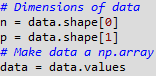
Splitting the dataset
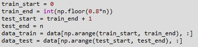
Next, we split the whole dataset into training and test data. The training data contained 1st 80% of the total dataset starting from 01 Jan 2000 and test data contained remaining 20% of data set. The data was not shuffled but sequentially sliced.
Scaling data & Building X, Y
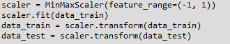
Another important step in data pre-processing is to standardize the dataset. This process makes the mean of all the input features equal to zero and also converts their variance to 1. This ensures that there is no bias while training the model due to the different scales of all input features. If this is not done the neural network might get confused and give a higher weight to those features which have a higher average value than others. Also, most common activation functions of the network’s neurons such as tanh or sigmoid are defined on the [-1, 1] or [0, 1] interval respectively. Nowadays, rectified linear unit (ReLU) activations are commonly used activations which are unbounded on the axis of possible activation values. However, we will scale both the inputs and targets. We will do Scaling using sklearn’s MinMaxScaler. We instantiate the variable sc with the MinMaxScalerr() function. After which we use the fit & then transform function train and test dataset.
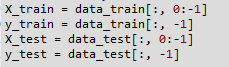
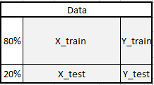
We then split the train and test dataset into Xtrain, ytrain & Xtest, ytest. This selects the target and predictors from datatrain and datatest. The target which is price rise (ytrain & ytest) is located in the last column of datatrain/test, the predictors which 8 features (Xtrain & Xtest) from 1st column to 8th column datatrain/test. The whole dataset will look like below.
This is an essential part of any machine learning algorithm, the training data is used by the model to arrive at the weights of the model. The test dataset is used to see how the model will perform on new data which would be fed into the model. The test dataset also has the actual value for the output, which helps us in understanding how efficient the model is. Now that the datasets are ready, we may proceed with building the Artificial Neural Network using the TensorFlow library.
Building The Artificial Neural Network
Input, Hidden & Output Layers
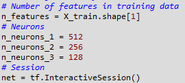
The model consists of three major building blocks. The input layer, the hidden layers and the output layer. The input layer is the 8 features. After input layers there are 3 hidden layers. The first hidden layer contains 512 neurons. Subsequent hidden layers are always half the size of the previous layer, which means 2nd hidden layers contains 256 and finally 3rd one 128 neurons. After 3 hidden layers there is output layer. Net is creating by tensor flow interactive secession.
Placeholders & Variables
The Artificial Neural Network starts with placeholders. We need two placeholders in order to fit our model contains the network's inputs (features of the stock at time T = t) and Y the network's output (Movement of the stock at T+1). The shape of the placeholders correspond to None, n_features with [None] meaning that the inputs are a 2-dimensional matrix and the outputs are a 1-dimensional vector. It is crucial to understand which input and output dimensions the neural net needs in order to design it properly. The none argument indicates that at this point we do not yet know the number of observations that flow through the neural net graph in each batch, so we keep if flexible. We will later define the variable batch size that controls the number of observations per training batch.
![]()
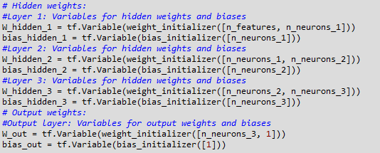
Besides placeholders, variables are another cornerstone of the TensorFlow universe. While placeholders are used to store input and target data in the graph, variables are used as flexible containers within the graph that are allowed to change during graph execution. Here Weights and Biases are represented as variables in order to adapt during training. Variables need to be initialized, prior to model training.
Initializers
Initializers are used to initialize the network’s variables before training. Since neural networks are trained using numerical optimization techniques, the starting point of the optimization problem is one the key factors to find good solutions to the underlying problem. There are different initializers available in Tensor flow, each with different initialization approaches. Here, we will use which is one of the default initialization strategies the tf.variancescalinginitializer() for two variables weight & bias.
![]()
Designing the network architecture
In designing the network architecture, 1st we need to understand the required variable dimensions between input, hidden and output layers. In case of multilayer perceptron (MLP), the network type we use here, the second dimension of the previous layer is the first dimension in the current layer for weight matrices. It means each layer passing its output as input to the next layer. The biases dimension equals the second dimension of the current layer’s weight matrix, which corresponds the number of neurons in this layer.
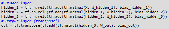
After definition of the required weight and bias variables, the network topology, the architecture of the network, needs to be specified. Hereby, placeholders (data) and variables (weights and biases) need to be combined into a system of sequential matrix multiplications. Furthermore, the hidden layers of the network are transformed by activation functions. Activation functions are important elements of the network architecture since they introduce non-linearity to the system. There are many possible activation functions out there, one of the most common is the rectified linear unit (ReLU) which will are using in this model.
Cost function
We use cost function to optimize the model. The cost function is used to generate a measure of deviation between the network’s predictions and the actual observed training targets. For regression problems, the mean squared error (MSE) function is commonly used. MSE computes the average squared deviation between predictions and targets.
![]()
Optimizer
The optimizer takes care of the necessary computations that are used to adapt the network’s weight and bias variables during training. Those computations invoke the calculation of gradients that indicate the direction in which the weights and biases have to be changed during training in order to minimize the network’s cost function. The development of stable and speedy optimizers is a major field in neural network and deep learning research.
![]()
In this model we use Adam (Adaptive Moment Estimation) Optimizer, which is an extension of the stochastic gradient descent, is one of the default optimizers in deep learning development.
Fitting the neural network
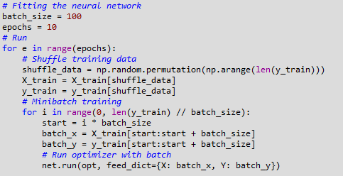
Now we need to fit the neural network that we have created to our train datasets. After having defined the placeholders, variables, initializers, cost functions and optimizers of the network, the model needs to be trained. Usually, this is done by mini batch training. During mini batch training random data samples of n = batchsize are drawn from the training data and fed into the network. The training dataset gets divided into n / batchsize batches that are sequentially fed into the network. At this point the placeholders X and Y come into play. They store the input and target data and present them to the network as inputs and targets.
A sampled data batch of X flows through the network until it reaches the output layer. There, TensorFlow compares the models predictions against the actual observed targets Y in the current batch. Afterwards, TensorFlow conducts an optimization step and updates the networks parameters, corresponding to the selected learning scheme. After having updated the weights and biases, the next batch is sampled and the process repeats itself. The procedure continues until all batches have been presented to the network. One full sweep over all batches is called an epoch. The training of the network stops once the maximum number of epochs is reached or another stopping criterion defined by the user applies. We stop the training network when epoch reaches 10.
With this, our artificial neural network has been compiled and is ready to make predictions.
Predicting The Movement Of The Stock
Now that the neural network has been compiled, we can use the predict() method for making the prediction. We pass Xtest as its argument and store the result in a variable named pred. We then convert pred data in to dataframe and saved in another variable called ypred. We then convert ypred to store binary values by storing the condition ypred >0.5. Now, the variable y_pred stores either True or False depending on whether the predicted value was greater or less than 0.5.
![]()
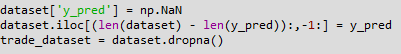
Next, we create a new column in the dataframe dataset with the column header ‘ypred’ and store NaN values in the column. We then store the values of ypred into this new column, starting from the rows of the test dataset. This is done by slicing the dataframe using the iloc method as shown in the code below. We then drop all the NaN values from dataset and store them in a new dataframe named trade_dataset.
Computing Strategy Returns
Now that we have the predicted values of the stock movement. We can compute the returns of the strategy. We will be taking a long position when the predicted value of y is true and will take a short position when the predicted signal is False.
We first compute the returns that the strategy will earn if a long position is taken at the end of today, and squared off at the end of the next day. We start by creating a new column named ‘Tomorrows Returns’ in the trade_dataset and store in it a value of 0. We use the decimal notation to indicate that floating point values will be stored in this new column. Next, we store in it the log returns of today, i.e. logarithm of the closing price of today divided by the closing price of yesterday. Next, we shift these values upwards by one element so that tomorrow’s returns are stored against the prices of today.

Next, we will compute the Strategy Returns. We create a new column under the header ‘StrategyReturns’ and initialize it with a value of 0. to indicate storing floating point values. By using the np.where() function, we then store the value in the column ‘Tomorrows Returns’ if the value in the ‘ypred’ column stores True (a long position), else we would store negative of the value in the column ‘Tomorrows Returns’ (a short position); into the ‘Strategy Returns’ column.

We now compute the cumulative returns for both the market and the strategy. These values are computed using the cumsum() function.
![]()
Plotting The Graph Of Returns
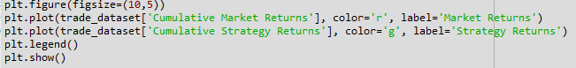
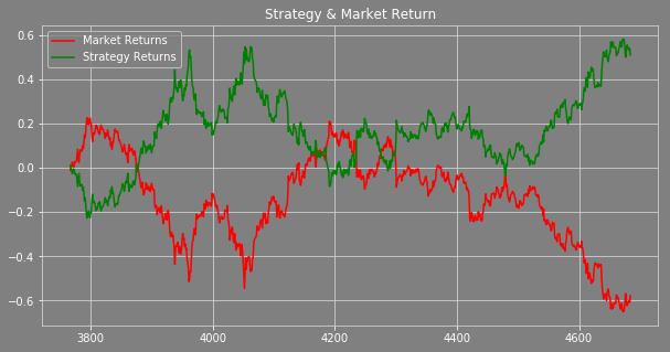
We will now plot the market returns and our strategy returns to visualize how our strategy is performing against the market. We then use the plot function to plot the graphs of Market Returns and Strategy Returns using the cumulative values stored in the dataframe trade_dataset. We then create the legend and show the plot using the legend() and show() functions respectively. The plot shown below is the output of the code. The green line represents the returns generated using the strategy and the red line represents the market returns.
Conclusion
The objective of this project is to make you understand how to build an artificial neural network using tensorflow in python and predicting stock price. The objective is not to show you to get a good return. You can optimize this model in various ways to get a good strategy return.
My advice is to use more than 100,000 data points when you are building Artificial Neural Network or any other Deep Learning model that will be most effective. This model was developed on daily prices to make you understand how to build the model. It is advisable to use the minute or tick data for training the model.
Now you can build your own Artificial Neural Network in Python and start trading using the power and intelligence of your machines.
You can also download the pyhon code and dataset from my github a/c
Next Step
Disclaimer: All investments and trading in the stock market involve risk. Any decisions to place trades in the financial markets, including trading in stock or options or other financial instruments is a personal decision that should only be made after thorough research, including a personal risk and financial assessment and the engagement of professional assistance to the extent you believe necessary. The trading strategies or related information mentioned in this article is for informational purposes only.
Download Data Files
- Deep Learning - Artificial Neural Network Using TensorFlow In Python