By Viraj Bhagat
The market progresses rapidly with trades executed in a mere fraction of time. Numerous traders and countless strategies play their part to be a part of this ride. At the end of the day, some stay afloat, while some steer upwards and some stumble or even fall to rise back up the next day. Learning about options trading plays a key role in this, as they provide the trader with the ability to create a variety and a number of strategies, but at the cost of time. The market is replete with many such strategies and it is essential that one spends time getting to learn them and study their technicalities. While stocks may allow one to trade only bearish or bullish, they often do move sideways but within a particular range. It is in such cases that one enters a Diagonal Spread.
What Are Spreads?
The simultaneous purchase and selling of security are called as a Spread or a Spread Trade or Relative Value Trade and are often executed with futures contracts and options as the legs. Securities besides these are also used sometimes. Spreads can be constructed with either calls or puts as either debit or credit spreads. Based on the relation of months and legs, the spread constructions are created and distinguished into Vertical Spreads, Horizontal Spreads and Diagonal Spreads.
What Are Diagonal Spreads?
Diagonal Spread Strategy is:
- An Options trading strategy
- A 2-step strategy
- Combines bits of both Long Call Calendar Spread and Short Call Spread
Comparison Of Vertical Spreads, Horizontal Spreads, and Diagonal Spreads
According to Investopedia, Diagonal Spread makes use of different months and strikes, it moves diagonally, and thus the name.

While it is stated that these were mentioned in the newspapers previously as:[1]
- Options Prices > Listed in Tabular Manner
- Strike Prices > Listed in Rows i.e. Vertically
- Expirations > Listed in Columns i.e. Horizontally
A Diagonal spread would thus mean presence of options in different row and columns with different strike prices and expiration dates.
Difference Between Calendar Spread And Diagonal Spread
The Diagonal Spread has a near-term outlook which could be bearish or bullish. It is similar to Calendar Spreads in the sense that:
- Near-term options are sold
- Long-term options are bought
- Take advantage of the rapid time decay in soon to expire options
What Is A Diagonal Call Spread?
When the Outlook is slightly bullish > One writes higher strike near-month calls > Against lower strike far-month calls
What Is A Diagonal Put Spread?
When the Outlook is slightly bearish > One writes lower strike near-month puts > Against higher strike far-month puts
When Is A Diagonal Spread Executed?
- A short-term weakness or Strength that you think would go up (if call) or go down again (if put), then to take advantage of it
- The strategy is controlled on the short-side for risk and if the market plays smooth, it can become open-ended on the long side
- When executed for money, it allows margin requirements to be met
- Short option expires ATM worthless > IV expands > Increases the price of the remaining Long Option> Keep full credit received to Sell the option > Reduces the cost basis of the long option we own
- Diagonal Spread > short side expires worthless > Money > Buy > Long side of the spread
Change Is The Key!
One must always be aware and be alert of the performance of his/her strategies. If in any case, the spread requires some adjustment, it would have to be taken care of to prevent any loss. One can use it as an advantage after the strategy has been implemented by consistently studying the market and implying the changes in their strategies to gain maximum benefit.
Profit From A Diagonal Spread Trading Strategy
The maximum profit of a Diagonal Spread can be described as follows:
- Max. Profit = Net credit received* - Premium paid for the call (with strike B)
- *Net credit is received by selling both calls with strike A)
Loss From A Diagonal Spread Trading Strategy
The maximum loss for a Diagonal Spread can be described as follows:
- For Net Credit: Max Loss = Strike A – Strike B – Net Credit Recd.
- For Net Debit: Max Loss = Strike A – Strike B + Net Debit Paid
Setup Of A Diagonal Spread Strategy
If the trade moves fast towards our direction, one could lose money. Thus, when compared to other spreads, the setup of a diagonal spread is very important. It involves the simultaneous purchase of:
- An equal number of options
- Both options should be of the same class
- Both should have the same underlying security
- 2 different strike prices
- 2 different expiration months
A Diagonal Spread for a Call would look like this: 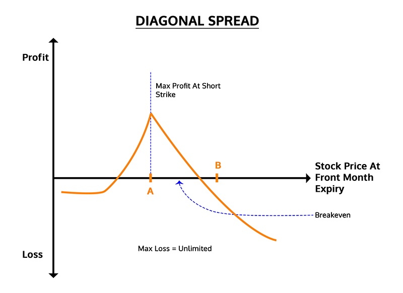
Strategy (In Case Of A ‘Call’)
- Sell 1 OTM Call – A – Lower Strike Price - Front-month
- Buy 1 OTM Call – B – Higher Strike Price – Back-month(Long-term)
- The stock generally will be below strike A
We will explain this strategy with the help of an Example.
Long Call Diagonal Spread
Implementing Long Call Diagonal Spread Trading Strategy
I would be explaining the example using Diagonal Spread with Long Calls and for this, I will use the example of NIFTY (Ticker – NIFTY) Following is the Option Chain for NIFTY  We would now take 2 Call Prices from April 2018 and May 2018 For April 2018:
  For May 2018:
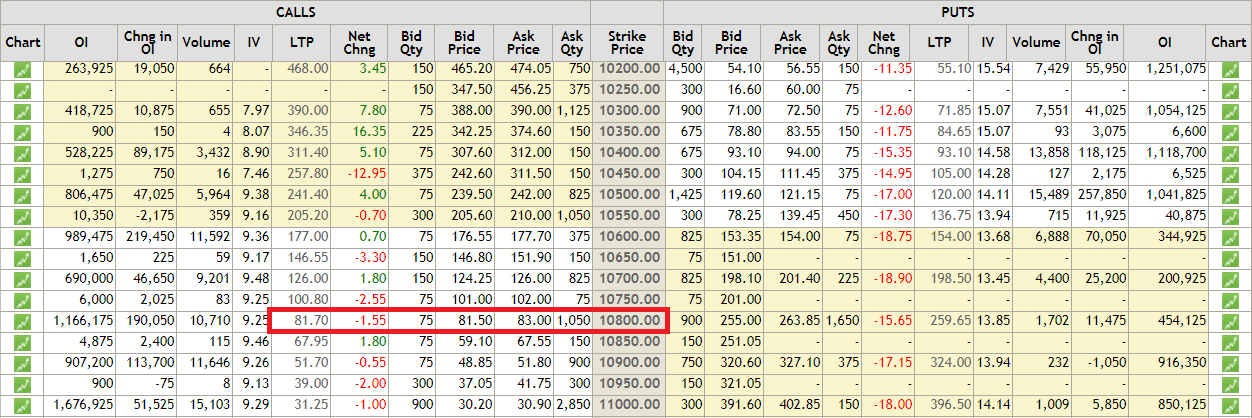
Strategy
# Importing Libraries
# Data manipulation
import numpy as np
import pandas as pd
# To plot
import matplotlib.pyplot as plt
import seaborn
plt.style.use('ggplot')
# BS Model
import mibian
# Importing Libraries
# Data manipulation
import numpy as np
import pandas as pd
# To plot
import matplotlib.pyplot as plt
import seaborn
plt.style.use('ggplot')
# BS Model
import mibian
# Nifty futures price
nifty_april_fut = 10595.40
nifty_may_fut = 10625.50
april_strike_price = 10700
may_strike_price = 10800
april_call_price = 10
may_call_price = 82
setup_cost = may_call_price - april_call_price
# Today's date is 20 April 2018. Therefore, days to April expiry is 7 days and days to May expiry is 41 days.
days_to_expiry_april_call = 6
days_to_expiry_may_call = 41
# Range of values for Nifty
sT = np.arange(0.97*nifty_april_fut,1.03*nifty_april_fut,1)
#interest rate for input to Black-Scholes model
interest_rate = 0.0
# Front-month IV
april_call_iv = mibian.BS([nifty_april_fut, april_strike_price, interest_rate, days_to_expiry_april_call],
callPrice=april_call_price).impliedVolatility
print "Front Month IV %.2f" % april_call_iv,"%"
# Back-month IV
may_call_iv = mibian.BS([nifty_may_fut, may_strike_price, interest_rate, days_to_expiry_may_call],
callPrice=may_call_price).impliedVolatility
print "Back Month IV %.2f" % may_call_iv,"%"
Front Month IV 8.53 %
Back Month IV 11.26 %
# Changing days to expiry to a day before the front-month expiry
days_to_expiry_april_call = 0.001
days_to_expiry_may_call = 35 - days_to_expiry_april_call
df = pd.DataFrame()
df['nifty_price'] = sT
df['april_call_price'] = np.nan
df['may_call_price'] = np.nan
# Calculating call price for different possible values of Nifty
for i in range(0,len(df)):
df.loc[i,'april_call_price'] = mibian.BS([df.iloc[i]['nifty_price'], april_strike_price, interest_rate, days_to_expiry_april_call],
volatility=april_call_iv).callPrice# Since, interest rate is considered 0%, 35 is added to the nifty price to get the Nifty December futures price.
df.loc[i,'may_call_price'] = mibian.BS([df.iloc[i]['nifty_price']+35, may_strike_price, interest_rate, days_to_expiry_may_call],
volatility=may_call_iv).callPrice
df.head()
nifty_price april_call_price may_call_price
0 10277.538 0.0 27.305711
1 10278.538 0.0 27.455138
2 10279.538 0.0 27.605211
3 10280.538 0.0 27.755935
4 10281.538 0.0 27.907309df['payoff'] = df.may_call_price - df.april_call_price - setup_cost
plt.figure(figsize=(10,5))
plt.ylabel("Payoff")
plt.xlabel("Nifty Price")
plt.plot(sT,df.payoff)
plt.show()
max_profit = max(df['payoff']) min_profit = min(df['payoff']) print "%.2f" %max_profit print "%.2f" %min_profit 35.55 -88.94
Maximum Profit: INR 35.55 Maximum Loss: INR -88.94
Conclusion
Seasoned Veterans and higher are mostly seen practising this strategy since it involves selling 2 options while having some volatility and predictability; yet having a steady stock price. One thus needs to be quite thorough with the market and his options to practise this strategy.
Modern trading demands a systematic approach and the need to steer yourself away from trading from the gut. Learn how you too can trade options in a systematic manner with our course on Systematic Options Trading. Plus, you get to explore explore options trading strategies like a butterfly, iron condor, and spread strategies. Enroll now!
Download Data File
- Diagonal Spread Options Strategy – Python Code
Disclaimer: All investments and trading in the stock market involve risk. Any decisions to place trades in the financial markets, including trading in stock or options or other financial instruments is a personal decision that should only be made after thorough research, including a personal risk and financial assessment and the engagement of professional assistance to the extent you believe necessary. The trading strategies or related information mentioned in this article is for informational purposes only.