
In this post, we will discuss on modeling option pricing using Black Scholes Option Pricing model and plotting the same for a combination of various options. If you are new to options trading then you can check the options trading basics guide to build your conceptual foundation before working with this Excel model. If you are new to options trading then you can check the options trading for dummies free course on Quantra. You can put any number of call and/or put o options in the model and use a built-in macro (named ‘BS’) for calculating the BS model based option pricing for each option. The macro (named ‘PayOff’) is used for plotting the Profit/Loss for the overall combination of the option positions against the spot price.
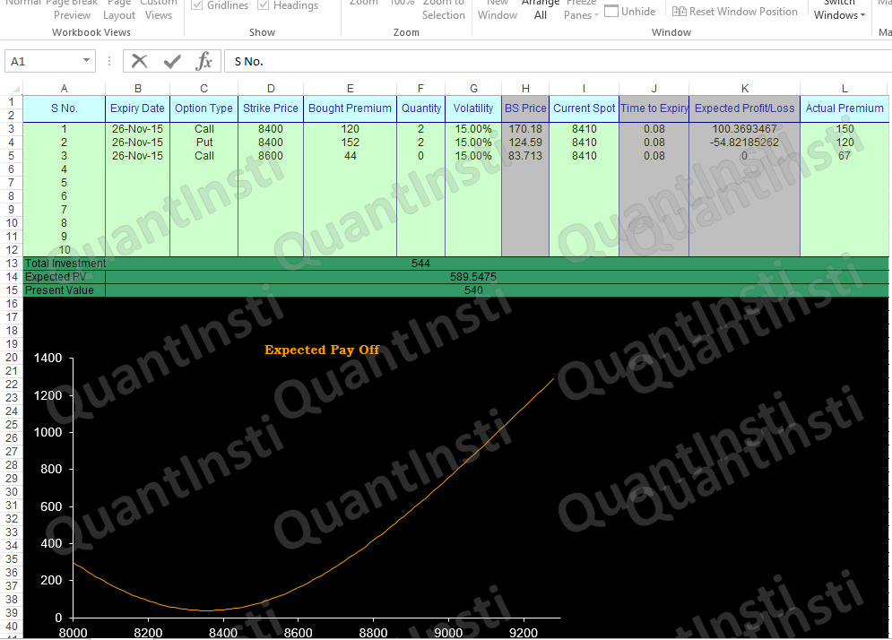
Sheet1 named Payoff has a table where we specify all option parameters. Column B specifies Expiry data for the options. Column C specifies the option type. Column D has the strike price of the underlying asset. Column E shows the premium amount in INR at which the option is bought. Column F tells us about the number of option contracts we have bought. Column G specifies the volatility, column H specifies Black Scholes price of the option (calculated by the macro “BS”. Column I is the current spot price of the underlying asset, column J shows the time to expiry of the option (calculated using the formula). Column K specifies the Expected PnL of the option (calculated using the formula). It is calculated as the difference between the Black Scholes price and the premium paid multiplied by the number of option contracts. Column L shows the actual premium in the market currently, meaning the current premium should you wish to buy the option.
The 13th row calculates the total investment. Since we have bought two calls and put options at a premium of 120 and 152 our total investment is 1202+1522=544. The 14th row shows the Expected present value. Since the market has moved after the options are bought, the current expected price of the option multiplied by the number of option contracts gives the expected value. Hence the expected payoff is 170.182+124.592=589.5475.
The present value in row 15 is calculated similarly by taking the product of actual premium in the market currently and the number of options contracts. Hence the present value is 1502+1202=540.
Plotting the Payoff
The graph below shows the plot of expected payoff for the option portfolio. This is done by taking the expected payoff values from sheet4. More on this later.
BS in Macros
BS Price sheet shows the pricing of an option using Black Scholes model. From Black-Scholes option pricing model, we know the price of a call option on a non-dividend stock can be written as:
$$ C_t = S_t N(d_1) - X e^{-r \tau} N(d_2) $$
The price of a put option on a non-dividend-paying stock is:
$$ P_t = X e^{-r \tau} N(-d_2) - S_t N(-d_1) $$
where:
$$ d_1 = \frac{\ln\left(\frac{S_t}{X}\right) + \left(r + \frac{\sigma_s^2}{2}\right)\tau}{\sigma_s \sqrt{\tau}} $$
$$ d_2 = d_1 - \sigma_s \sqrt{\tau} $$
$$ \tau = T - t $$
Here, the terms are defined as follows:
- \( S_t \) - Current price of the underlying asset
- \( X \) - Strike price
- \( r \) - Risk-free interest rate
- \( \tau \) - Time to expiry
- \( \ln \) - Natural logarithm
The call and put value using Black Scholes framework is calculated in the 13th and 14th row for the parameters specified in row 1 to 5.

Customizing BS
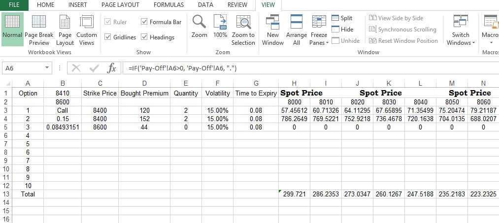
“Back-end BS” sheet has the same set of values of Payoff sheet from columns A to G. Column H onwards shows the spot price ranges in the 2nd row. You can change the starting point for the price range of Spot Price in Cell H2. The increment (presently of 10 points) can be changed from Cell I2 and then drag it across the range horizontally. The 3rd row shows the Black Scholes call option for the specified parameters and varying spot price. The 4th row shows the Black Scholes put option for the specified parameters and varying spot price. Please note that though the post shows the calculation for three options, you can go up to 10 options combinations of by just filling appropriate values in the table in Sheet1. For more than 10 options, you can edit the sheet and the macro.
The 13th row calculates the total payoff from the option position. This is calculated as the difference between the profits from options and the total investment.
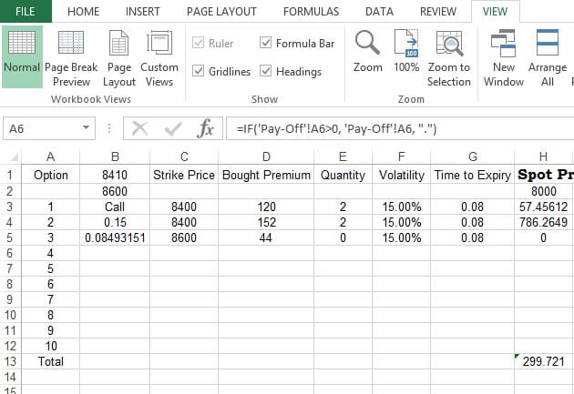
In this case, the profit from overall option position is the sum of H3 and H4. The total investment (calculated in Payoff Sheet 13th row) of 544 has to be subtracted from the sum of H3 and H4 to obtain the final payoff. Similar calculations are done to all other columns henceforth.
The Expected Payoff graph in Sheet1 is the plot of total payoff calculated in Sheet3 against the underlying spot price.

There are two macros. One in BS Price sheet that calculates Black Scholes option price depending upon the values entered in the Payoff sheet. The other one is in the Payoff sheet that plots the Expected Payoff graph. Please make a note that the Expiry Date in Payoff sheet is set beyond the current date, else the Black Scholes price will not return a numerical value for a negative time period.
You can enroll for this free online python course on Quantra and understand basic terminologies and concepts that will help you trade in options.
Next Step
In our next post, we have covered the basics of Bull Call Spread Option strategy, includes a bonus Python code and Excel model that shows how to implement this strategy using a live example.
Modern trading demands a systematic approach and the need to steer yourself away from trading from the gut. This course on Systematic Options Trading helps you create, backtest, implement, live trade and analyse the performance of options strategy
Disclaimer: All investments and trading in the stock market involve risk. Any decisions to place trades in the financial markets, including trading in stock or options or other financial instruments is a personal decision that should only be made after thorough research, including a personal risk and financial assessment and the engagement of professional assistance to the extent you believe necessary. The trading strategies or related information mentioned in this article is for informational purposes only.
Download Excel Model