
In today’s algorithmic trading having a trading edge is one of the most critical elements. It’s plain simple. If you don’t have an edge, don’t trade! Hence, as a quant, one is always on a lookout for good trading ideas. One of the good resources for quantitative trading strategies that have been gaining wide popularity is the Quantpedia site. Quantpedia has thousands of financial research papers that can be utilized to create profitable trading strategies.

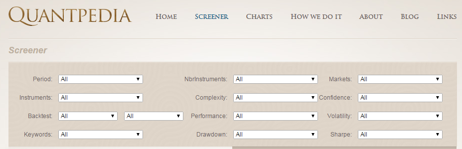
The “Screener” page on Quantpedia categorizes hundreds of trading strategies based on different parameters like Period, Instruments, Markets, Complexity, Performance, Drawdown, Volatility, Sharpe etc.
Quantpedia has made some of these trading strategies available for free to their users. In this article, we will explore one such trading strategy listed on their site called the “52-Weeks High Effect in Stocks”.
52-Weeks High Effect in Stocks
The Quantpedia page[1] for this trading strategy provides a detailed description which includes the 52-weeks high effect explanation, source research paper, other related papers, a visualization of the strategy performance and also other related trading strategies.
What is 52-Weeks High Effect?
Let us put down the lucid explanation provided on Quantpedia here -
The “52-week high effect” states that stocks with prices close to the 52-week highs have better subsequent returns than stocks with prices far from the 52-week highs. Investors use the 52-week high as an “anchor” which they value stocks against. When stock prices are near the 52-week high, investors are unwilling to bid the price all the way to the fundamental value. As a result, investors’ under-react when stock prices approach the 52-week high, and this creates the 52-week high effect.
Source Paper
The Source paper[2], “Industry Information and the 52-Week High Effect” has been authored by Xin Hong, Bradford D. Jordan, and Mark H. Liu.
The financial paper says that traders use the 52-week high as a reference point which they evaluate the potential impact of news against. When good news has pushed a stock’s price near or to a new 52-week high, traders are reluctant to bid the price of the stock higher even if the information warrants it. The information eventually prevails and the price moves up, resulting in a continuation. It works similarly for 52-week lows.
The trading strategy developed by the authors buys stocks in industries in which stock prices are close to 52-week highs and shorts stocks in industries in which stock prices are far from 52-week highs. They found that the industry 52-week high trading strategy is more profitable than the individual 52-week high trading strategy proposed by George and Hwang (2004).
Framing our 52-Weeks High Effect Strategy using R programming
Having understood the 52-weeks High Effect, we will try to backtest a simple trading strategy using R programming. Please note that we are not trying to replicate the exact trading strategy developed by the authors in their research paper.
We test our trading strategy for a 3-year backtest period using daily data on around 140 stocks listed on the National Stock Exchange of India Ltd. (NSE).
Brief about the strategy
The trading strategy reads the daily historical data for each stock in the list and checks if the price of the stock is near its 52-week high at the start of each month. We have shown how to check for this condition in step 4 of the trading strategy formulation process illustrated below. For all the stocks that pass this condition, we form an equal-weighted portfolio for that month. We take a long position in these stocks at the start of the month and square off our position at the start of the next month. We follow this process for every month of our backtest period. Finally, we compute and chart the performance metrics of our trading strategy.
The course provides a comprehensive guide to backtesting such strategies, helping you implement and test them with historical data. Through backtesting, you can evaluate the effectiveness of your strategy and refine it for better performance in future market conditions.
Now, let us understand the process of trading strategy formulation in a step-by-step manner. For reference, we have posted the R code snippets of relevant sections of the trading strategy under its respective step.
The process of trading strategy formulation
Step 1
First, we set the backtest period, and the upper and lower thresholds values for determining whether a stock is near its 52-week high.
# Setting the lower and upper threshold limits
lower_threshold_limit = 0.90 # (eg.0.90 = 90%)
upper_threshold_limit = 0.95 # (eg.0.95 = 95%)
# Backtesting period (Eg. 1 = 1 year) minimum period selected should be 2 years.
noDays = 4
Step 2
In this step, we read the historical stock data using the read.csv function from R. We are using the data from Google finance and it consists of the Open/High/Low/Close (OHLC) & Volume values.
# Run the program for each stock in the list
for(s in 1:length(symbol)){

print(s)

dirPath = paste(getwd(),"/4 Year Historical Data/",sep="")
fileName = paste(dirPath,symbol[s],".csv",sep="")
data = as.data.frame(read.csv(fileName))
data$TICKER = symbol[s]}
# Merge NIFTY prices with Stock data and select the Close Price
data = merge(data,data_nifty, by = "DATE")
data = data[, c("DATE", "TICKER","CLOSE.x","CLOSE.y")]
colnames(data) = c("DATE","TICKER","CLOSE","NIFTY")
N = nrow(data)
Step 3:
Since we are using the daily data we need to determine the start date of each month. The start date need not necessarily be the 1st of every month because the 1st can be a weekend or a holiday for the stock exchange. Hence, we write an R code which will determine the first date of each month.
# Determine the date on which each month of the backtest period starts

data$First_Day = ""

day = format(ymd(data$DATE),format="%d")
monthYr = format(ymd(data$DATE),format="%Y-%m")
yt = tapply(day,monthYr, min)

first_day = as.Date(paste(row.names(yt),yt,sep="-"))
frows = match(first_day, ymd(data$DATE))
for (f in frows) {data$First_Day[f] = "First Day of the Month"}

data = data[, c("TICKER","DATE", "CLOSE","NIFTY","First_Day")]
Step 4:
Check if the stock is near the 52-week high mark. In this part, we first compute the 52-week high price for each stock. We then compute the upper and the lower thresholds using the 52-week high price.
Example:
If the lower threshold = 0.90, upper threshold = 0.95 and the 52-week high = 1200, then the threshold range is given by:
Threshold range = (0.90 * 1200) – (0.95 * 1200)
Threshold range = 1080 to 1140
If the stock price at the start of the month falls in this range, we then consider the stock to be near its 52-week high mark. We have also included one additional condition in the step. This condition checks whether the stock price in the past 30 days had reached the current 52-week high price and whether it is within the threshold range now. Such a stock will not be included in our portfolio as we assume that the stock price is in decline after reaching today’s 52-week high price.
# Check if the stock is near its 52-week high at the start of the each month

data$Near_52_Week_High = "" ; data$Max_52 = numeric(nrow(data));
data$Max_Not = numeric(nrow(data));

frows_tp = frows[frows >= 260]
for (fr in frows_tp){

   # This will determine the max price in the last 1 year (252 trading days)
   data$Max_52[fr] = max(data$CLOSE[(fr-252):(fr-1)])

  # This will check whether the max price has occurred in the last "x" days.
  data$Max_Not[fr] = max(data$CLOSE[(fr-no_max):(fr-1)])

  if ((data$CLOSE[fr] >= lower_threshold_limit * data$Max_52[fr])
      & (data$CLOSE[fr] <= upper_threshold_limit * data$Max_52[fr])
      & (data$Max_Not[fr] != data$Max_52[fr]) == TRUE ){
  data$Near_52_Week_High[fr] = "Near 52-Week High"
  } else {
  data$Near_52_Week_High[fr] = "Not Near 52-Week High"
  }

}
Step 5:
For all the stocks that fulfil the criteria mentioned in the step above, we create a long-only portfolio. The entry price equals the price at the start of the month. We square off our long position at the start of the next month. We consider the close price of the stock for our entry and exit trades.
# Enter into a long position for stocks at each start of month

data = subset(data,select=c(TICKER,DATE,CLOSE,NIFTY,First_Day,Max_52,Near_52_Week_High)
             ,subset=(First_Day=="First Day of the Month"))
data$NEXT_CLOSE = lagpad(data$CLOSE, 1)
colnames(data) = c("TICKER","DATE","CLOSE","NIFTY","First_Day","Max_52","Near_52_Week_High",
                   "NEXT_CLOSE")


data$Profit_Loss = numeric(nrow(data)); data$Nifty_change = numeric(nrow(data));

for (i in 1:length(data$CLOSE)) {
  if ((data$Near_52_Week_High[i] == "Near 52-Week High") == TRUE){
  data$Profit_Loss[i] = round(data$CLOSE[i+1] - data$CLOSE[i],2)
  data$Nifty_change[i] = round(Delt(data$NIFTY[i],data$NIFTY[i+1])*100,2)
  }
}

for (i in 1:length(data$CLOSE)) {
  if ((data$Near_52_Week_High[i] == "Not Near 52-Week High") == TRUE){
  data$Profit_Loss[i] = 0
  data$Nifty_change[i] = round(Delt(data$NIFTY[i],data$NIFTY[i+1])*100,2)
  }

}
Step 6:
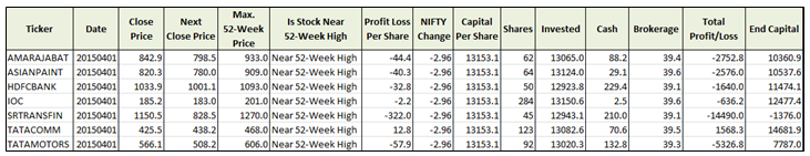
In this step, we write an R code which creates a summary sheet of all the trades for each month in the backtest period. A sample summary sheet has been shown below. It also includes the Profit/Loss from every trade undertaken during the month.
# Create a Summary worksheet for all the trades during a particular month

final_data = final_data[-1,]
final_data = subset(final_data,select=c(TICKER,DATE,CLOSE,NEXT_CLOSE,Max_52,
                                        Near_52_Week_High,Profit_Loss,Nifty_change),
                                        subset=(Near_52_Week_High == "Near 52-Week High"))

colnames(final_data) = c("Ticker","Date","Close_Price","Next_Close_Price",
                         "Max. 52-Week price","Is Stock near 52-Week high",
                         "Profit_Loss","Nifty_Change")

merged_file = paste(date_values[a],"- Summary.csv")
write.csv(final_data,merged_file)
Step 7:
In the final step, we compute the portfolio performance over the entire backtest period and also plot the equity curve using the PerformanceAnalytics package in R. The portfolio performance is saved in a CSV file.
cum_returns = Return.cumulative(eq_ts, geometric = TRUE)
print(cum_returns)

charts.PerformanceSummary(eq_ts,geometric=TRUE, wealth.index = FALSE)
print(SharpeRatio.annualized(eq_ts, Rf = 0, scale = 12, geometric = TRUE))
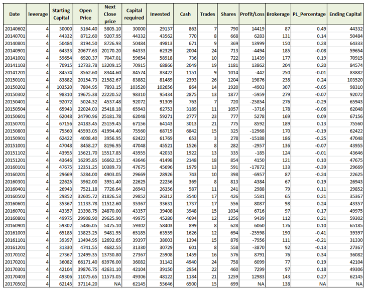
A sample summary of the portfolio performance has been shown below. In this case, the input parameters to our trading strategy were as follows:
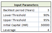
 Plotting the Equity Curve
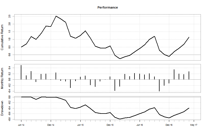
As can be observed from the equity curve, our trading strategy performed well during the initial period and then suffered drawdowns in the middle of the backtest period. The Sharpe ratio for the trading strategy comes to 0.4098.
Cumulative Return 1.172446

Annualized Sharpe Ratio (Rf=0%) 0.4098261
This was a simple trading strategy that we developed using the 52-week high effect explanation. One can tweak this trading strategy further to improve its performance and make it more robust or try it out in different markets.
Next Step
Access the final project submitted by Gopal as a part of his coursework in Executive Programme in Algorithmic Trading (EPAT) at QuantInsti. The project covers the trend following strategy based on the indicators like MACD, SuperTrend, and ADX coded in Python.
Update
We have noticed that some users are facing challenges while downloading the market data from Yahoo and Google Finance platforms. In case you are looking for an alternative source for market data, you can use Quandl for the same.
Disclaimer: All investments and trading in the stock market involve risk. Any decisions to place trades in the financial markets, including trading in stock or options or other financial instruments is a personal decision that should only be made after thorough research, including a personal risk and financial assessment and the engagement of professional assistance to the extent you believe necessary. The trading strategies or related information mentioned in this article is for informational purposes only.