By José Carlos Gonzáles Tanaka
In the first part of my ARMA article series, I covered the background theory of lag operators, the stationarity and invertibility of Autoregressive Moving Average models (ARMA) and the different types of versions you can create from it. Here, we’ll explore theoretically these models using Python. You'll learn about ARMA model Python examples. From the simulation of these models to a trading strategy based on these models.
It covers:
- Simulation of ARMA models in Python
- Autocovariance and autocorrelation functions of the ARMA models in Python
- An ARMA-based trading strategy in Python
Simulation of ARMA models in Python
Let’s first code some ARMA simulations to learn how the Autocorrelation functions (ACF) and Partial autocorrelation functions (PACF) behave.
Setting up the environment
First, we import the necessary libraries:
Simulation of ARMA models
Now, we set the seed and the input parameters
In the following code, we create some simulated ARMA models, specifically:
- AR(1) or ARMA(1,0) models with phis equal to (0.1, 0.25, 0.5, 0.75, 0.9, 0.99)
- MA(1) or ARMA(0,1) models with thetas equal to (-0.1, -0.25, -0.5, -0.75, -0.9, -0.99)
- An ARMA(1,1) model with phi and theta both equal to 0.3.
- We have 13 models in total.
ARMA model simulation graphs
We code the ARMA models’ time series graphs
We get them as below:

As you can see, as we increase the phi value, we have a more random walk process, i.e. a less stationary process. Let’s see what happens with the ACFs and PACFs.
Autocovariance and autocorrelation functions of the ARMA models in Python
This section will help you understand the Box-Jenkins methodology, described in part 1.
ARMA(1,0)s Autocorrelation Functions
Let’s code to output the ACFs and PACFs for each AR(1) model.
So we can get the ACFs’ and PACFs’ graphs below
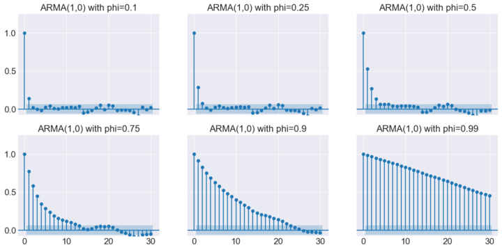

You can get some conclusions:
- For all the AR(1) models, the PACFs are significant up to lag 1.
- ACFs are significant for many lags and decay gradually.
- However, as phi increases, the ACFs start to decay less rapidly.
- So, if you have a random walk process, you might expect its ACFs will take many lags to decay, while a stationary process with a low phi value will have its ACF decay rapidly.
Let’s see, for the MA(1) processes, their ACFs and PACFs. We have first the code:
ARMA(1,0)s Partial Autocorrelation Functions
And then the graphs:


Some conclusions:
- For all the MA(1) models, the ACFs are significant up to lag 1.
- PACFs are significant for many lags and decay gradually.
- However, as theta increases, the PACFs start to decay less rapidly.
- So, if you have a non-invertible process, you might expect its PACFs will take many lags to decay, while an invertible process with a low theta value will have its PACF decay rapidly.
The general conclusions are explained in point 2 of the Brief on Box-Jenkins methodology.
An ARMA-based trading strategy in Python
So, instead of using the Box-Jenkins methodology, which requires checking the plot of the ACF and PACF of the plausible models to fit them with your time series, you can use the Akaike's information criterion (AIC) to choose the best model.
Time Series Analysis
Financial Time Series Analysis for Smarter Trading
This procedure is usually done by practitioners whenever they want to estimate an ARMA model algorithmically. Let's do some ARMA model forecasting!
We’re going to use the same libraries we imported previously and import the AAPL data from yahoo finance.
Next, we compute the first and second differences of the Apple series.
We do this because we need to find first the order of integration of the Apple time series, as below
As you see, only the prices in levels are a random walk. Consequently, the AAPL time series behaves as I(1). So, in order to create our ARMA model, we will use the first difference of the time series.
Now, we create some dictionaries, lists, dataframes and variables to create a loop later.
The loop procedure consists of estimating 35 models with p and q going from 0 to 5 (the ARMA(0,0) is ignored since this is just a random process). You will choose the best ARMA model for each day from October 2021 to August 2023. The best model will be the one with the lowest AIC.
Once you estimate the best model on each day, you will forecast with that model what the return would be on the next day. If the forecast return is positive, you will go long, if it’s negative, you will go short. You repeat this whole process for each day until August 26th, 2023.
Then, we compute the strategy returns:
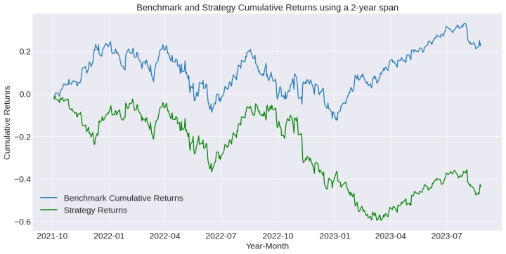
Finally, we plot the strategy and buy-and-hold returns:
We use 2 spans: A 1-year span and a 2-year span.
Check the cumulative returns on each case:

Some suggestions:
- You need to optimize the estimation historical data span to have a better strategy performance
- You can use a risk management process to improve the performance
- Short selling might be quite complex in stock trading. Please modify the code as needed to make a proper short-selling backtesting code.
Conclusion
In this write-up, you learned how to code an ARMA model in Python you created a strategy based on it. We didn’t take into account commissions and slippage. Be careful about them. Don’t forget to implement a risk management process so you can improve the results.
This model is an econometric model. Do you want to learn more about this topic and other algo trading models? Don’t hesitate to subscribe to our course Algorithmic Trading for Beginners! This learning track uses Python for many strategies. You’ll benefit a lot from it!
Files in the download:
- Python codes used in the blog
Disclaimer: All investments and trading in the stock market involve risk. Any decision to place trades in the financial markets, including trading in stock or options or other financial instruments is a personal decision that should only be made after thorough research, including a personal risk and financial assessment and the engagement of professional assistance to the extent you believe necessary. The trading strategies or related information mentioned in this article is for informational purposes only.