Stationarity: Defining, Detecting, Types, and Transforming Time Series

By Satyapriya Chaudhari

When dealing with a time series data, you would often come across two terms - stationary time series and non-stationary time series. Stationarity is one of the key components in time series analysis.

In this blog, you will read about the below topics.

• Definition of Stationarity
• Stationary Time Series and Non-Stationary Time Series
• Importance of Stationarity
• Types of Stationarity
• Detecting Stationarity
• Transforming a Non-Stationary Series into a Stationary Series

Let us begin by understanding what is a stationary process.

Definition of Stationarity

As defined in Wikipedia ⁽¹⁾, a stationary process is “a process whose unconditional joint probability distribution does not change when shifted in time.”

This means that the distribution of a stationary process would look the same at different points in time. As a result, the parameters of a stationary process, like mean and variance, remain constant over time.

So if you have a process with, let’s suppose, one hundred values. You sample values from 1 to 30 or 30 to 50 or 50 to 100. In order for this process to be stationary, the mean and other statistical properties of different samples should be approximately the same.

Stationarity is one of the key components in time series analysis. Take a pause and think why? We will come back to this after looking at the stationary and non-stationary time series.

Stationary Time Series and Non-Stationary Time Series

A time series whose statistical properties, such as mean, variance, etc., remain constant over time, are called a stationary time series.

In other words, a stationary time series is a series whose statistical properties are independent of the point in time at which they are observed. A stationary time series has a constant variance and it always returns to the long-run mean.

A time series whose statistical properties change over time is called a non-stationary time series. Thus a time series with a trend or seasonality is non-stationary in nature. This is because the presence of trend or seasonality will affect the mean, variance and other properties at any given point in time.

Let’s summarise the differences between a stationary time series and a non-stationary time series.

Importance of Stationarity

Remember we left a question, “Why is stationarity one of the key components in time series analysis?”

Before you answer that, what will happen if a process is not stationary?

Yes, the inferences drawn from a non-stationary process will not be reliable as its statistical properties will keep on changing with time. While performing analysis, you would typically be interested in the expected value of the mean, the variance, etc.

But if these parameters are continuously changing, estimating them by averaging over time will not be accurate. Hence, stationary data are easier to analyse and any forecast made using a non-stationary data would be erroneous and misleading.

Because of this, many statistical procedures applied in time series analysis makes an assumption that the underlying time series data is stationary.

This assumption is necessary because most time series forecasting methods predict the statistical properties of the time series will remain the same in the future as they have been in the past.

Let’s move to the type of stationarity.

Types of Stationarity

Different types of stationarity are as follows.

• Strict stationarity - This means that the unconditional joint distribution of any moments (e.g. expected values, variances, third-order and higher moments) remains constant over time. This type of series is rarely seen in real-life practice.
• First-order stationarity - These series have a mean constant over time. Any other statistics (like variance) can change at the different points in time.
• Second-order stationarity (also called weak stationarity) - These time series have a constant mean and variance over time. Other statistics in the system are free to change over time. This is one of the most commonly observed series in real-life practice.
• Trend stationarity - These series are the series with a trend. This trend when removed from the series leaves a stationary series.
• Difference stationarity - These series are the series that need one or more differencing to become stationary. We will look into this in detail later in the article.

Detecting Stationarity

Since many analytical tools and statistical tests assume the time series to be stationary, it is very important to ascertain whether a given series is generated by a stationary process. Below are certain ways to do the same.

Visualization

The most common method to check whether a given data comes from a stationary series or not is by simply plotting the data or some function of it. Let us now see how these techniques can help us identify stationarity.

• Looking at the Data - Both stationary and non-stationary series have some properties that can be detected very easily from the plot of the data. For example, in a stationary series, the data points would always return towards the long-run mean with a constant variance. In a non-stationary series, the data points might show some trend or seasonality. Let us take a reference of the series of plots from the website, Forecasting: Principles and Practice by Hyndman & Athanasopoulos, 2018 ⁽²⁾.

Figure: Nine examples of time series data

1. 1. Google stock price for 200 consecutive days
   2. Daily change in the Google stock price for 200 consecutive days
   3. Annual number of strikes in the US
   4. Monthly sales of new one-family houses sold in the US
   5. Annual price of a dozen eggs in the US (constant dollars)
   6. Monthly total of pigs slaughtered in Victoria, Australia
   7. Annual total of lynx trapped in the McKenzie River district of north-west Canada
   8. Monthly Australian beer production
   9. Monthly Australian electricity production

From the nine plots in the figure above, which ones do you think are stationary series?

The series (b) is stationary. You can check the explanation here ⁽³⁾. This method is only used to get an initial insight into the data and is not completely reliable.

• Looking at the Autocorrelation Functions plots - Let us see the ACF plot of the series (a) and series (b) from above. Here you will get to know what AutoCovariance and AutoCorrelation ⁽⁴⁾ functions are.

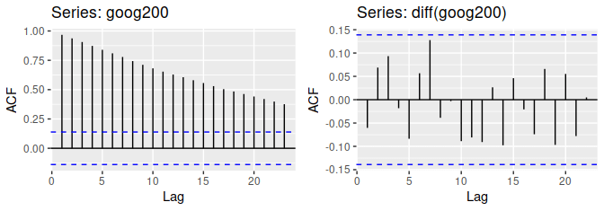
Figure:

1. 1. ACF plot of Google stock price for 200 consecutive days.
   2. ACF plot of Daily change in the Google stock price for 200 consecutive days.

You already know that the series (a) is non-stationary and the series (b) is stationary.

What are your observations from the two plots above?

The value of ACF for lag 1 in the first plot is very high, close to one and it decreases very slowly. This is the case of a non-stationary series. However, in the second plot, that is for a stationary series, the value of the ACF for lag 1 is very small, and it drops to zero quickly.

Thus, for a stationary series, the value of the ACF for lag 1 is large and positive. And for a non-stationary series, it is close to zero. For a non-stationary series, the value of ACF drops to zero relatively quickly.

Let us see another example. We will read the Google stock price data from yfinance.com from January 2019 to April 2020 and visualise the series.

What do you think of the above series? Is it stationary?

No. The series has the data at different levels showing different trends. Hence, it does not seem to be stationary.

You learned how you can visually check the data for stationarity. Let’s move ahead to another technique to analyse if a data is stationary.

Summary Statistics

You already know that a stationary time series has a constant mean, variance, etc. over time. Summary statistics like mean and variance are thus helpful in estimating whether a time series is stationary or not.

You can partition the data into random periods and analyse the summary statistics for different periods. If the mean and variance of different partitions are very close to each other, the series is stationary.

If there is a significant difference between the mean and variance of the different partitions, then the series is not stationary.

Let us split the Google price data we saw above into halves and analyse the statistics.

The output of the above code is

You can see that both the values of the two means and the two variances differ significantly. This again suggests that the series is not stationary.

You compared the summary statistics of the different partitions of the data for stationarity. A more reliable and convenient method to check the stationarity of a series is the different statistical tests that can be performed on the data to check if they are generated from a stationary process or not.

Statistical Tests

A number of parametric and nonparametric tests are available to check for the stationarity of the series. Let's have a look at a couple of parametric tests and their Python implementation.

• Augmented Dickey-Fuller Test - The Augmented Dickey-Fuller test is one of the most popular tests to check for stationarity. It tests the below hypothesis.
• Null Hypothesis, H0: The time series is not stationary.
• Alternative Hypothesis, H1: The time series is stationary.

You can use the adfuller method from the statsmodels library to perform this test in Python and compare the value of the test statistics or the p-value.

• If the p-value is less than or equal to 0.05 or the absolute value of the test statistics is greater than the critical value, you reject H0 and conclude that the time series is stationary.
• If the p-value is greater than 0.05 or the absolute value of the test statistics is less than the critical value, you fail to reject H0 and conclude that the time series is not stationary.

Let’s see how you can implement this in Python.

The result is returned in the form of a tuple. You can see the result in the below format.

The output of the code is as below.

As you can see, the p-value is greater than 0.05. You fail to reject the null hypothesis and conclude that the time series is not stationary.

Alternatively, you can compare the ADF test statistics to the critical value. Since the absolute value of ADF test statistics is less than the absolute value of the critical value, you fail to reject the null hypothesis and conclude that the time series is not stationary.

• Kwiatkowski-Phillips-Schmidt-Shin test - Another quite commonly used test for stationarity is the KPSS test. A very important point to note here is that the interpretation of KPSS is entirely opposite of the ADF test, and hence these tests cannot be used interchangeably. One needs to be very careful while interpreting these tests. KPSS test tests the below hypothesis.
• Null Hypothesis, H0: The time series is stationary.
• Alternative Hypothesis, H1: The time series is not stationary.

You can use the kpss method from the statsmodels library to perform this test in Python and compare the value of the test statistics or the p-value. Since the hypothesis is the opposite of that you saw in the ADF test, the interpretation of the p-value is also opposite.

• If the p-value is less than or equal to 0.05 or the absolute value of the test statistics is greater than the critical value, you reject H0 and conclude that the time series is not stationary.
• If the p-value is greater than 0.05 or the absolute value of the test statistics is less than the critical value, you fail to reject H0 and conclude that the time series is stationary.

Let’s see how you can implement this in Python.

The result is returned in the form of a tuple. You can see the result in the below format.

The output of the code is as below.

As you can see, the p-value is less than 0.05. You reject the null hypothesis and conclude that the time series is not stationary. This is consistent with the result obtained with the ADF test.

Apart from these parametric tests, there are other semi-parametric and non-parametric tests also available to check for the stationarity of a series. These tests are beyond the scope of this article.

Transforming a Non-Stationary Series into a Stationary Series

Since stationary series are easy to analyze, you can convert a non-stationary series into a stationary series by the method of Differencing. In fact, it is necessary to convert a non-stationary series into a stationary series in order to use time series forecasting models.

In this method, the difference of consecutive terms in the series is computed as below.

Let us compute the difference of the Google price series and plot the result.

Let’s apply the ADF test on the differenced series and check if the series is stationary or not.

The output of the above code is

As you can see, the p-value is less than 0.05. You reject the null hypothesis and conclude that the time series is stationary.

Thus, the Google price series was a difference-stationary series. The first-order difference of the Google price series resulted in a stationary series.

Suggested Reads

• All about Time Series
• Augmented Dickey-Fuller Test

You can watch the video below on stationarity for more understanding.

Conclusion

Stationarity is one of the key components in time series analysis. A stationary times series is independent of the point in time where it is observed. Most of the forecasting models in time series assume the underlying time series to be stationary. Hence, for the forecast to be reliable, it is necessary for the time series to be stationary.

You can use different techniques to check whether a given time series is stationary or not.  Most of the time series data in financial markets are far from stationary and thus have to be transformed into a stationary series before making predictions.

To know more about stationary and non-stationary time series data, and various time series analysis models, check out our course on Financial Time Series Analysis for Trading.

Disclaimer: All investments and trading in the stock market involve risk. Any decisions to place trades in the financial markets, including trading in stock or options or other financial instruments is a personal decision that should only be made after thorough research, including a personal risk and financial assessment and the engagement of professional assistance to the extent you believe necessary. The trading strategies or related information mentioned in this article is for informational purposes only.