
This post on Bayesian inference is the second of a multi-part series on Bayesian statistics and methods used in quantitative finance.
In my previous post, I gave a leisurely introduction to Bayesian statistics and while doing so distinguished between the frequentist and the Bayesian outlook of the world. I dwelt on how each of their underlying philosophies influenced their analysis of various probabilistic phenomena. I then discussed the Bayes' Theorem along with some illustrations to help lay the building blocks of Bayesian statistics.
Intent of this Post
My objective here is to help develop a deeper understanding of statistical analysis by focusing on the methodologies adopted by frequentist statistics and Bayesian statistics. I consciously choose to tackle the programming and simulation aspects using Python in my next post.
I now instantiate the previously discussed ideas with a simple coin-tossing example adapted from "Introduction to Bayesian Econometrics (2nd Edition)".
Example: A Repeated Coin-Tossing Experiment
Suppose we are interested in estimating the bias of a coin whose fairness is unknown. We define θ (the Greek letter 'theta') as the probability of getting a head after a coin is tossed. θ is the unknown parameter we want to estimate. We intend to do so by inspecting the results of tossing the coin multiple times. Let us denote y as a realization of the random variable Y (representing the outcome of a coin toss). Let Y=1 if a coin toss results in heads and Y=0 if a coin toss results in tails. Essentially, we are assigning 1 to heads and 0 to tails.
∴ P(Y=1|θ)=θ ; P(Y=0|θ)=1−θ
Based on our above setup, Y can be modelled as a Bernoulli distribution which we denote as
Y ∼ Bernoulli (θ)
I now briefly view our experimental setup through the lens of the frequentist and the Bayesian before proceeding with our estimation of the unknown parameter θ.
Two Perspectives on the Experiment Setup
In classical statistics (i.e. the frequentist approach), our parameter θ is a fixed but unknown value lying between 0 and 1. The data we collect is one realization of a recurrent (i.e. repeating this n-toss experiment say N times) experiment. Classical estimation techniques like the method of maximum likelihood are used to arrive at θ̄̂ (called 'theta hat'), an estimate for the unknown parameter θ. In statistics, we usually express an estimate by putting a hat over the name of the parameter. I dilate this idea in the next section. To restate what has been said previously, we observe that in the frequentist universe, the parameter is fixed but the data is varying.
Bayesian statistics is fundamentally different. Here, the parameter θ is treated as a random variable since there is uncertainty about its value. It, therefore, makes sense for us to regard our parameter as a random variable which will have an associated probability distribution. In order to apply Bayesian inference, we turn our attention to one of the fundamental laws of probability theory, Bayes' Theorem that we had seen previously.
I use the mathematical form of Bayes' Theorem as a way to establish a connection with Bayesian inference.
 ……..
……..  (1)
(1)
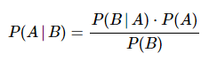
To repeat what I said in my previous post, what makes this theorem so handy is it allows us to invert a conditional probability. So if we observe a phenomenon and collect data or evidence about it, the theorem helps us analytically define the conditional probability of different possible causes given the evidence.
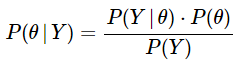
Let's now apply this to our example by using the notations we had defined earlier. I label A = θ and B = y. In the field of Bayesian statistics, there are special names used for each of these terms which I spell out below and use subsequently. (1) can be rewritten as:
 …….. (2)
where:
P(θ) is the prior probability. We express our belief about the cause θ BEFORE observing the evidence Y. In our example, the prior would be quantifying our a priori belief on the fairness of the coin (here we can start with the assumption that it is an unbiased coin, so θ = 1/2). P(Y|θ) is the likelihood. Here is where the real action happens. This is the probability of the observed sample or evidence given the hypothesized cause. Let us, without loss of generality, assume that we obtain 5 heads in 8 coin tosses. Presuming the coin to be unbiased as specified above, the likelihood would be the probability of observing 5 heads in 8 tosses given that θ = 1/2. P(θ|Y) is the posterior probability. This is the probability of the underlying cause θ AFTER observing the evidence y. Here, we compute our updated or a posteriori belief on the bias of the coin after observing 5 heads in 8 coin tosses using Bayes' theorem. P(Y) is the probability of the data or evidence. We sometimes also call this the marginal likelihood. This is obtained by taking the weighted sum (or integral) of the likelihood function of the evidence across all possible values of θ. In our example, we would compute the probability of 5 heads in 8 coin tosses for all possible beliefs about θ. This term is used to normalize the posterior probability. Since it is independent of the parameter to be estimated θ, it is mathematically more tractable to express the posterior probability as:
P(θ|Y) ∝ P(Y|θ) × P(θ) …….(3)
(3) is the most important expression in Bayesian statistics and bears repeating. For clarity, I paraphrase what I said earlier. Bayesian inference allows us to turnaround conditional probabilities i.e. use the prior probabilities and the likelihood functions to provide a connecting link to the posterior probabilities i.e. P(θ|Y) granted that we only know P(Y|θ) and the prior, P(θ). I find it helpful to view (3) as:
Posterior Probability ∝ Likelihood × Prior Probability ………. (4)
The experimental objective is to get an estimate of the unknown parameter θ based on the outcome of n independent coin tosses. The coin tosses generate the sample or data y = (y1, y2, …, yn), where yi is 1 or 0 based on the result of the ith coin toss.
I now show the frequentist and Bayesian approaches to fulfilling this objective. Feel free to cursorily skim through the derivations I touch upon here if you are not interested in the mathematics behind it. You can still develop sufficient intuitions and learn to use Bayesian techniques in practice.
Estimating θ: The Frequentist Approach
We compute the joint probability function using the maximum likelihood estimation (MLE) approach. The probability of the outcome for a single coin toss can be elegantly expressed as:
![]()
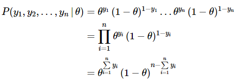
For a given value of θ, the joint probability of the outcome for n independent coin tosses is the product of the probability of each individual outcome:
 ……. (5)
As we can see in (4), the expression worked out is a function of the unknown parameter θ given the observations from our experiment. This function of θ is called the likelihood function and is usually referred to in the literature as:
![]() ……….. (6)
……….. (6)
OR
![]() …………… (7)
…………… (7)
We would like to compute the value of θ which is most likely to have yielded the observed set of outcomes. This is called the maximum likelihood estimate, θ̄̂ ('theta hat'). For analytically computing it, we trivially take the first order derivative of (6) with respect to the parameter and set it equal to zero. It is prudent to also take the second derivative and check the sign of its value at θ = θ̄̂ to ensure that the estimate is indeed the maxima. We often customarily take the log of the likelihood function since it greatly simplifies the determination of the maximum likelihood estimator θ̄̂ . It should therefore not surprise you that the literature is replete with log likelihood functions and their solutions.
Estimating θ: The Bayesian Approach
I now change the notations we have used so far to make them a little more precise mathematically. I will use these notations throughout this series now. The reason for this alteration is so that we can suitably ascribe each term with symbols that remind us of their random nature. There is uncertainty over the values of θ, Y, etc., we, therefore, regard them as random variables and assign them corresponding probability distributions which I do below.
Notations for the Density and Distribution Functions
- π(⋅) (the Greek letter 'pi') to denote the probability distribution function of the prior (this is pertaining to θ) and π(⋅|y) to denote the posterior density function of the parameter we attempt to estimate.
- f(⋅) to denote the probability density function (pdf) for continuous random variables and p(.) which is the probability mass function (pmf) of discrete random variables. However, for simplicity, I use f(⋅) irrespective of whether the random variable Y is continuous or discrete.
- The joint density function will continue to be denoted as L(θ|⋅). to denote the likelihood function which is the joint density of the sample values and is usually the product of the pdf's/pmf's of the sample values from our data.
Remember that θ is the parameter we are trying to estimate.
(2) and (3) can be rewritten as
π(θ|y) = [f(y|θ)⋅π(θ)] / f(y) ……(8)
π(θ|y)∝f(y|θ)×π(θ) …………….(9)
Stated in words, the posterior distribution function is proportional to the likelihood function times the prior distribution function. I redraw your attention to (4) and present it in congruence with our new notations.
Posterior PDF ∝ Likelihood × Prior PDF ……….(10)
I now rewrite (8) and (9) using the likelihood function L(θ|Y) defined earlier in (7).
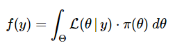
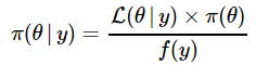 ……… (11)
![]() ………..(12)
………..(12)
The denominator of (11) is the probability distribution of the evidence or data. I reiterate what I have previously mentioned while inspecting (3): A useful way of considering the posterior density is using the proportionality approach as seen in (12). That way, we don't need to worry about the f(y) term on the RHS of (11).
For the mathematically curious among you, I now take you briefly down a needless rabbit hole to explain it incompletely. Perhaps, later in our journey, I may write a separate post brooding on these minutiae.
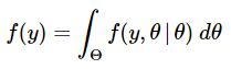
In (11), f(y) is the proportionality constant that makes the posterior distribution a proper density function integrating to 1. When we examine it more closely, we see that is, in fact, the unconditional (marginal) distribution of the random variable Y. We can determine it analytically by integrating over all possible values of the parameter θ. Since we are integrating out θ, we find that f(y) does not depend on θ.
OR
(11) and (12) represent the continuous versions of the Bayes' Theorem.
The posterior distribution is central to Bayesian statistics and inference because it blends all the updated information about the parameter θ in a single expression. This includes information about θ before the observations were inspected and this is captured through the prior distribution. The information contained in the observations is captured through the likelihood function.
We can regard (11) as a method of updating information and this idea is further exemplified by the prior-posterior nomenclature.
- The prior distribution of θ, π(θ) represents the information available about its possible values before recording the observations y.
- The likelihood function L(θ|y) of θ is then determined based on the observations y.
- The posterior distribution of θ, π(θ|y) summarizes all the available information about the unknown parameter θ after recording and incorporating the observations y.
The Bayesian estimate of θ would be the weighted average of the prior estimate and the maximum likelihood estimate, θ̄̂ . As the number of observations n increases and approached infinity, the weight on the prior estimate approaches zero and the weight on the MLE approaches one. This implies that the Bayesian and frequentist estimates would converge as our sample size gets larger.
To clarify, in a classical or frequentist setting, the usual estimator of the parameter, θ is the ML estimator, θ̄̂ . Here, the prior is implicitly treated as a constant.
Summary
I have devoted this post to deriving the fundamental result of Bayesian statistics, viz. (10) . The essence of this expression is to represent uncertainty by combining the knowledge obtained from two sources - observations and prior beliefs. In doing so, I introduced the concepts of prior distributions, likelihood functions and posterior distributions as well as the comparison of the frequentist and Bayesian methodologies. In my next post, I intend to make good my promise of illustrating the above example with simulations in Python.
Bayesian statistics is an important part of quantitative strategies which are part of an algorithmic trader’s handbook. The Executive Programme in Algorithmic Trading (EPAT™) course by QuantInsti® covers training modules like Statistics & Econometrics, Financial Computing & Technology, and Algorithmic & Quantitative Trading that equip you with the required skill sets for applying various trading instruments and platforms to be a successful trader.
Disclaimer: All investments and trading in the stock market involve risk. Any decisions to place trades in the financial markets, including trading in stock or options or other financial instruments is a personal decision that should only be made after thorough research, including a personal risk and financial assessment and the engagement of professional assistance to the extent you believe necessary. The trading strategies or related information mentioned in this article is for informational purposes only.
