
By Vivek Krishnamoorthy and Aacashi Nawyndder
TL;DR
Bayesian statistics offers a flexible, adaptive framework for making trading decisions by updating beliefs with new market data. Unlike traditional models, Bayesian methods treat parameters as probabilities, making them ideal for uncertain, fast-changing financial markets. Understanding Bayesian methods is increasingly seen as a core competency in quant trading, where probabilistic thinking drives better decision-making.
They’re used in risk management, model tuning, classification, and incorporating expert views or alternative data. Tools like PyMC and Bayesian optimisation make it accessible for quants and traders aiming to build smarter, data-driven strategies.
This blog covers:
- The Bayesian Basics
- Why Bayesian Statistics Shines in Algorithmic Trading
- Practical Bayesian Applications in Algorithmic Trading
- Recent Industry Buzz in Bayesian Algorithmic Trading
- The Upsides and Downsides: What to Keep in Mind
- Frequently Asked Questions
Want to ditch rigid trading models and truly harness the power of incoming market information? Imagine a system that learns and adapts, just like you do, but with the precision of mathematics. Welcome to the world of Bayesian statistics, a game-changing framework for algorithmic traders. It’s all about making informed decisions by logically blending what you already know with what the market is telling you right now.
Let's explore how this can sharpen your trading edge!
This approach contrasts with the traditional, or "frequentist," view of probability, which often sees probabilities as long-run frequencies of events and parameters as fixed, unknown constants (Neyman, 1937).
Bayesian statistics, on the other hand, treats parameters themselves as random variables about which we can have beliefs and update them as more data comes in (Gelman et al., 2013). Honestly, this feels tailor-made for trading, doesn't it? After all, market conditions and relationships are hardly ever set in stone. So, let's jump in and see how you can use Bayesian stats to get a leg up in the fast-paced world of finance and algorithmic trading.
Prerequisites
To fully grasp the Bayesian methods discussed in this blog, it is important to first establish a foundational understanding of probability, statistics, and algorithmic trading.
For a conceptual introduction to Bayesian statistics, Bayesian Inference Methods and Equation Explained with Examples offers an accessible explanation of Bayes' Theorem and how it applies to uncertainty and decision-making, foundational to applying Bayesian models in markets.
What You'll Learn:
- The core idea behind Bayesian thinking is updating beliefs with new evidence.
- Understanding Bayes' Theorem: your mathematical tool for belief updating.
- Why Bayesian methods are a great fit for the uncertainties of financial markets.
- Practical examples of Bayesian statistics in algorithmic trading:
- Estimating model parameters that adapt to new data.
- Building simple predictive models (like Naive Bayes for market direction).
- Incorporating expert views or alternative data into your models.
- The Pros, Cons, and Recent Trends of Using Bayesian Approaches in Quantitative Finance.
The Bayesian Basics
Prior Beliefs, New Evidence, Updated Beliefs
Okay, let's break down the fundamental magic of Bayesian statistics. At its core, it's built on a wonderfully simple yet incredibly powerful idea: our understanding of the world is not static; it evolves as we gather more information.
Think about it like this: you've got a new trading strategy you're mulling over.
- Prior Belief (Prior Probability): Based on your initial research, backtesting on historical data, or even a hunch, you have some initial belief about how profitable this strategy might be. Let's say you think there's a 60% chance it will be profitable. This is your prior.
- New Evidence (Likelihood): You then deploy the strategy on a small scale or observe its hypothetical performance over a few weeks of live market data. This new data is your evidence. The likelihood function tells you how probable this new evidence is, given different underlying states of the strategy's true profitability.
- Updated Belief (Posterior Probability): After observing the new evidence, you update your initial belief. If the strategy performed well, your confidence in its profitability might increase from 60% to, say, 75%. If it performed poorly, it might drop to 40%. This updated belief is your posterior.
This whole process of tweaking your beliefs based on new info is neatly wrapped up and formalised by what is called the Bayes' Theorem.
Bayes' Theorem: The Engine of Bayesian Learning
So, Bayes' Theorem is the actual formula that ties all these pieces together. If you have a hypothesis (let’s call it H) and some evidence (E), the theorem looks like this:
Bayes’ Theorem:
\( P(H \mid E) = \frac{P(E \mid H) \cdot P(H)}{P(E)} \)
Where:
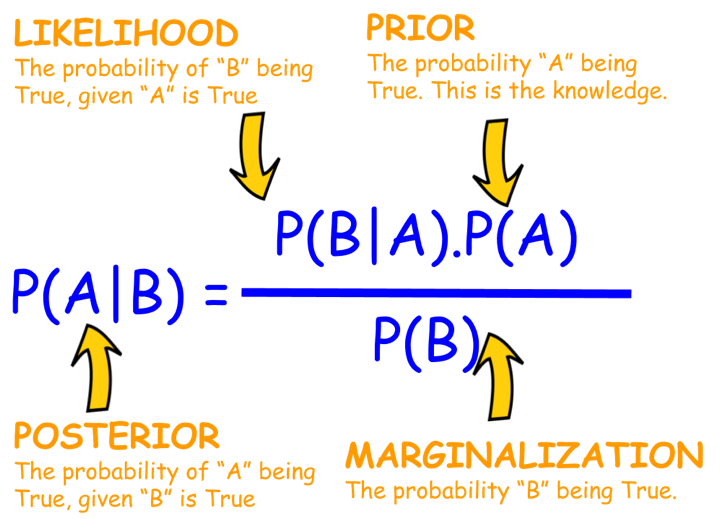
- P(H|E) is the Posterior Probability: The probability of your hypothesis (H) being true after observing the evidence (E). This is what you want to calculate; your updated belief.
- P(E|H) is the Likelihood: The probability of observing the evidence (E) if your hypothesis (H) were true. For example, if your hypothesis is “this stock is bullish,” how likely is it to see a 2% price increase today?
- P(H) is the Prior Probability: The probability of your hypothesis (H) being true before observing the new evidence (E). This is your initial belief.
- P(E) is the Probability of the Evidence (also called Marginal Likelihood or Normalising Constant): The overall probability of observing the evidence (E) under all possible hypotheses. It's calculated by summing (or integrating) P(E|H) × P(H) over every possible H. This ensures the posterior probabilities sum up to 1.
Let's try to make this less abstract with a quick trading scenario.
Example: Is a News Event Bullish for a Stock?
Suppose a company is about to release an earnings report.
- Hypothesis (H): The earnings report will be significantly better than expected (a "positive surprise").
- Prior P(H): Based on analyst chatter and recent sector performance, you believe there's a 30% chance of a positive surprise. So, P(H) = 0.30.
- Evidence (E): In the hour before the official announcement, the stock price jumps 1%.
- Likelihood P(E|H): You know from past experience that if there's a genuinely positive surprise brewing, there's a 70% chance of seeing such a pre-announcement price jump due to insider information or some sharp traders catching on early. So, P(E|H) = 0.70.
- Probability of Evidence P(E): This one's a little more involved because the price could jump for other reasons, too, right? Maybe the whole market is rallying, or it's just a false rumour. Let's say:
- The probability of the price jump if it's a positive surprise (P(E|H)) is 0.70 (as above).
- The probability of the price jump if it's not a positive surprise (P(E|not H)) is, say, 0.20 (it's less likely, but possible).
- Since P(H) = 0.30, then P(not H) = 1 - 0.30 = 0.70.
- So, P(E) = P(E|H)P(H) + P(E|not H)P(not H) = (0.70 * 0.30) + (0.20 * 0.70) = 0.21 + 0.14 = 0.35.
Now we can calculate the Posterior \( P(H \mid E) \):
\( P(H \mid E) = \frac{0.70 \times 0.30}{0.35} = \frac{0.21}{0.35} = 0.60 \)
Boom! After seeing that 1% price jump, your belief that the earnings report will be a positive surprise has shot up from 30% to 60%! This updated probability can then inform your trading decision, perhaps you're now more inclined to buy the stock or adjust an existing position.
Of course, this is a super-simplified illustration. Real financial models are juggling a significantly greater number of variables and much more complex probability distributions. But the beautiful thing is, that core logic of updating your beliefs as new info comes in? That stays exactly the same.
Why Bayesian Statistics Shines in Algorithmic Trading
Financial markets are a wild ride, full of uncertainty, constantly changing relationships (non-stationarity, if you want to get technical), and often, not a lot of data for those really rare, out-of-the-blue events. Bayesian methods offer several advantages in this environment:
- Handles Uncertainty Like a Pro: Bayesian statistics doesn't just give you a single number; it naturally deals with uncertainty by using probability distributions for parameters, instead of pretending they are fixed, known values (Bernardo & Smith, 2000). This gives you a much more realistic picture of what might happen.
- Updating Beliefs with New Data: Algorithmic trading systems constantly process new market data. Bayesian updating allows models to adapt dynamically. For instance, the volatility of an asset isn't constant; a Bayesian model can update its volatility estimate as new price ticks arrive.
- Working with Small Data Sets: Traditional frequentist methods often require large sample sizes for reliable estimates. Bayesian methods, however, can give you pretty sensible insights even with limited data, because they let you bring in "informative priors" – basically, your existing knowledge from experts, similar markets, or financial theories (Ghosh et al., 2006). This is a lifesaver when you're trying to model rare events or new assets that don't have a long history.
- Model Comparison and Averaging: Bayesian techniques provide a really solid way (e.g., using Bayes factors or posterior predictive checks) to compare different models and even average out their predictions. This often leads to more robust and reliable results (Hoeting et al., 1999).
- Lets You Weave in Qualitative Insights: Got a strong economic reason why a certain parameter should probably fall within a specific range? Priors give you a formal way to mix that kind of qualitative hunch or expert opinion with your hard quantitative data.
- Clearer Interpretation of Probabilities: When a Bayesian model tells you "there's a 70% chance this stock will go up tomorrow," it means exactly what it sounds like: it’s your current degree of belief. This can be a lot more straightforward to act on than trying to interpret p-values or confidence intervals alone (Berger & Berry, 1988).
Practical Bayesian Applications in Algorithmic Trading
Alright, enough theory! Let's get down to brass tacks. How can you actually use Bayesian statistics in your trading algorithms?
1. Adaptive Parameter Estimation: Keeping Your Models Fresh
So many trading models lean heavily on parameters – like the lookback window for your moving average, the speed of mean reversion in a pairs trading setup, or the volatility guess in an options pricing model. But here’s the catch: market conditions are always shifting, so parameters that were golden yesterday might be suboptimal today.
This is where Bayesian methods are super handy. They let you treat these parameters not as fixed numbers, but as distributions that get updated as new data rolls in. Imagine you're estimating the average daily return of a stock.
- Prior: You might start with a vague prior idea(e.g., a normal distribution centred around 0 with a wide spread (standard deviation)) or a more educated guess based on how similar stocks in the sector have performed historically.
- Likelihood: As each new trading day provides a return, you calculate the likelihood of observing that return given different possible values of the true average daily return.
- Posterior: Bayes' theorem combines the prior and likelihood to give you an updated distribution for the average daily return. This posterior becomes the prior for the next day's update.It's a continuous learning loop!
Hot Trend Alert: Techniques like Kalman Filters (which are inherently Bayesian) are widely used for dynamically estimating unobserved variables, like the "true" underlying price or volatility, in noisy market data (Welch & Bishop, 2006). Another area is Bayesian regression, where the regression coefficients (e.g., the beta of a stock) are not fixed points but distributions that can evolve.
For more on regression in trading, you might want to check out how Regression is Used in Trading.
Simplified Python Example: Updating Your Belief about a Coin's Fairness (Think Market Ups and Downs)
Let's say we want to get a handle on the probability of a stock price going up (we'll call it 'Heads') on any given day. This is a bit like trying to figure out if a coin is fair or biased.
Python Code:
Output:
Initial Prior: Alpha=1, Beta=1
Observed Data: 6 'up' days, 4 'down' days
Posterior Belief: Alpha=7, Beta=5
Updated Estimated Probability of an 'Up' Day: 0.58
95% Credible Interval for p_up: (0.31, 0.83)
In this code:
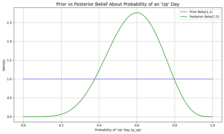
- We start off with a Beta(1,1) prior, which is uniform and suggests any probability of an 'up' day is equally likely.
- Then, we observe 10 days of market data with 6 'up' days.
- The posterior distribution becomes Beta(1+6, 1+4) = Beta(7, 5).
- Our new point estimate for the probability of an 'up' day is 7 / (7+5) = 0.58, or 58%.
- The credible interval gives us a range of plausible values.
The graph provides a clear visual for this belief-updating process. The flat blue line represents our initial, uninformative prior, where any probability for an 'up' day was considered equally likely. In contrast, the orange curve is the posterior belief, which has been sharpened and informed by the observed market data. The peak of this new curve, centered around 0.58, represents our updated, most probable estimate, while its more concentrated shape signifies our reduced uncertainty now that we have evidence to guide us.
This is a toy example, but it shows the mechanics of how beliefs get updated. In algorithmic trading, this could be applied to the probability of a profitable trade for a given signal or the probability of a market regime persisting.
2. Naive Bayes Classifiers for Market Prediction: Simple but Surprisingly Smart!
Next up, let's talk about Naive Bayes. It's a straightforward probabilistic classifier that uses Bayes' theorem, but with a "naive" (or let's say, optimistic) assumption that all your input features are independent of each other. Despite its simplicity, it can be surprisingly effective for tasks like classifying whether the next day's market movement will be 'Up', 'Down', or 'Sideways' based on current indicators. (Rish, 2001)
Here’s how it works (conceptually):
- Define Features: These could be technical indicators (e.g., RSI < 30, MACD crossover), price patterns (e.g., yesterday was an engulfing candle), or even sentiment scores from financial news.
- Collect Training Data: Gather historical data where you have these features and the actual outcome (Up/Down/Sideways).
- Calculate Probabilities from Training Data:
- Prior Probabilities of Outcomes: P(Up), P(Down), P(Sideways) – simply the frequency of these outcomes in your training set.
- Likelihood of Features given Outcomes: P(Feature_A | Up), P(Feature_B | Up), etc. For instance, "What's the probability RSI < 30, given the market went Up the next day?"
- Make a Prediction: For new data (today's features):
- Calculate the posterior probability for each outcome:
- P(Up | Features) ∝ P(Up) * P(Feature_A | Up) * P(Feature_B | Up) * ...
- P(Down | Features) ∝ P(Down) * P(Feature_A | Down) * P(Feature_B | Down) * ...
- (And similarly for Sideways)
- The outcome with the highest posterior probability is your prediction.
Python Snippet Idea (Just a concept, you'd need sklearn for this):
Python Code:
Output:
Naive Bayes Classifier Accuracy (on dummy data): 0.43
This accuracy score of 0.43 indicates the model correctly predicted the market's direction 43% of the time on the unseen test data. Since this result is below 50% (the equivalent of random chance), it suggests that, with the current dummy data and features, the model does not demonstrate predictive power. In a real-world application, such a score would signal that the chosen features or the model itself may not be suitable, prompting a re-evaluation of the approach or further feature engineering.
This little snippet gives you the basic flow. Building a real Naive Bayes classifier for trading takes careful thought about which features to use (that's "feature engineering") and rigorous testing (validation). That "naive" assumption that all features are independent might not be perfectly true in the messy, interconnected world of markets, but it often gives you a surprisingly good starting point or baseline model.
Curious about where to learn all this? Don’t worry, friend, we’ve got you covered! Check out this course.
3. Bayesian Risk Management (e.g., Value at Risk - VaR)
You've probably heard of Value at Risk (VaR), it's a common way to estimate potential losses. But traditional VaR calculations can sometimes be a bit static or rely on simplistic assumptions. Bayesian VaR allows for the incorporation of prior beliefs about market volatility and tail risk, and these beliefs can be updated as new market shocks occur. This can lead to risk estimates that are more responsive and robust, especially when markets get choppy.
For instance, if a "black swan" event occurs, a Bayesian VaR model can adapt its parameters much more quickly to reflect this new, higher-risk reality. A purely historical VaR, on the other hand, might take a lot longer to catch up.
4. Bayesian Optimisation for Finding Goldilocks Strategy Parameters
Finding those "just right" parameters for your trading strategy (like the perfect entry/exit points or the ideal lookback period) can feel like searching for a needle in a haystack. Bayesian optimisation is a seriously powerful technique that can help here. It cleverly uses a probabilistic model (often a Gaussian Process) to model the objective function (like how profitable your strategy is for different parameters) and selects new parameter sets to test in a way that balances exploration (trying new areas) and exploitation (refining known good areas) (Snoek et al., 2012). This can be much more efficient than just trying every combination (grid search) or picking parameters at random.
Hot Trend Alert:Bayesian optimisation is a rising star in the broader machine learning world and is incredibly well-suited for fine-tuning complex algorithmic trading strategies, especially when running each backtest takes a lot of computational horsepower.
5. Weaving in Alternative Data and Expert Hunches (Opinions)
These days, quants are increasingly looking at "alternative data" sources, things like satellite images, the general mood on social media, or credit card transaction trends. Bayesian methods give you a really natural way to integrate such diverse and often unstructured data with traditional financial data. You can set your priors based on how reliable or strong you think the signal from an alternative data source is.
And it's not just about new data types. What if a seasoned portfolio manager has a strong conviction about a particular sector because of some geopolitical development that's difficult to quantify? That "expert opinion" can actually be formalised into a prior distribution, allowing it to influence the model's output right alongside the purely data-driven signals.
Recent Industry Buzz in Bayesian Algorithmic Trading
While Bayesian methods have been around in finance for a while, a few areas are really heating up and getting a lot of attention lately:
- Bayesian Deep Learning (BDL): You know how traditional deep learning models give you a single prediction but don't really tell you how "sure" they are? BDL is here to change that! It combines the power of deep neural networks with Bayesian principles to produce predictions with associated uncertainty estimates (Neal, 1995; Gal & Ghahramani, 2016). This is crucial for financial applications where knowing the model's confidence is as important as the prediction itself. For example, imagine a BDL model not just predicting a stock price, but also saying it's "80% confident the price will land between X and Y".
- Probabilistic Programming Languages (PPLs): Languages like Stan, PyMC3 (Salvatier et al., 2016), and TensorFlow Probability are making it easier for quants to build and estimate complex Bayesian models without getting bogged down in the low-level mathematical details of inference algorithms like Markov Chain Monte Carlo (MCMC). This easier access is really democratising the use of sophisticated Bayesian techniques across the board (Carpenter et al., 2017).
- Sophisticated MCMC and Variational Inference: As our models get more ambitious, the computational grunt work needed to fit them also grows. Thankfully, researchers are constantly cooking up more efficient MCMC algorithms (like Hamiltonian Monte Carlo) and speedier approximate methods like Variational Inference (VI) (Blei et al., 2017), making larger Bayesian models tractable for real-world trading.
If you want to learn more about MCMC, QuantInsti has an excellent blog on Introduction to Monte Carlo Analysis. - Dynamic Bayesian Networks for Spotting Market Regimes: Financial markets often seem to flip between different "moods" or "regimes", think high-volatility vs. low-volatility periods, or bull vs. bear markets. Dynamic Bayesian Networks (DBNs) can model these hidden market states and the probabilities of transitioning between them, allowing strategies to adapt their behavior accordingly (Murphy, 2002).
The Upsides and Downsides: What to Keep in Mind
Like any powerful tool, Bayesian methods come with their own set of pros and cons.
Advantages:
- Intuitive framework for updating beliefs.
- Quantifies uncertainty directly.
- Works well with limited data by using priors.
- Allows incorporation of expert knowledge.
- Provides a coherent way to compare and combine models.
Limitations:
- Choice of Prior: The selection of a prior can be subjective and can significantly influence the posterior, especially with small datasets. A poorly chosen prior can lead to poor results. While techniques for "objective" or "uninformative" priors exist, their appropriateness is often debated.
- Computational Cost: For complex models, estimating the posterior distribution (especially using MCMC methods) can be computationally intensive and time-consuming, which might be a constraint for high-frequency trading applications.
- Mathematical Complexity: While PPLs are helpful, a solid understanding of probability theory and Bayesian concepts is still needed to apply these methods correctly and interpret results.
Frequently Asked Questions
Q. What makes Bayesian statistics different from traditional (frequentist) methods in trading?
Bayesian statistics treats model parameters as random variables with a and allows beliefs to be updated with new data. In contrast, frequentist methods assume parameters are fixed and require large data samples. Bayesian thinking is more dynamic and well-suited to the non-stationary, uncertain nature of financial markets.
Q. How does Bayes’ Theorem help in trading decisions? Can you give an example?
Bayes’ Theorem is used to update probabilities based on new market information. For example, if a stock price jumps 1% before earnings, and past data suggests this often precedes a positive surprise, Bayes’ Theorem helps revise your confidence in that hypothesis, turning a 30% belief into 60%, which can directly influence your trade.
Q. What are priors and posteriors in Bayesian models, and why do they matter in finance?
A prior reflects your initial belief (from past data, theory, or expert views), while a posterior is the updated belief after considering new evidence. Priors help improve performance in low-data or high-uncertainty situations and allow integration of alternative data or human intuition in financial modelling.
Q. What types of trading problems are best suited for Bayesian methods?
Bayesian techniques are ideal for:
- Parameter estimation that adapts (example, volatility, beta, moving average lengths)
- Market regime detection using dynamic Bayesian networks
- Risk management (example, Bayesian VaR)
- Strategy optimisation using Bayesian Optimisation
- Classification tasks with Naive Bayes models
These approaches help build more responsive and robust strategies.
Q. Can Bayesian methods work with limited or noisy market data?
Yes! Bayesian methods shine in low-data environments by incorporating informative priors. They also handle uncertainty naturally, representing beliefs as distributions rather than fixed values, crucial when modelling rare market events or new assets.
Q. How is Bayesian optimisation used in trading strategy design?
Bayesian optimisation is used to tune strategy parameters (like entry/exit thresholds) efficiently. Instead of brute-force grid search, it balances exploration and exploitation using a probabilistic model (example, Gaussian Processes), making it perfect for costly backtesting environments.
Q. Are simple models like Naive Bayes really useful in trading?
Yes, Naive Bayes classifiers can serve as lightweight baseline models to predict market direction using indicators like RSI, MACD, or sentiment scores. While the assumption of independent features is simplistic, these models can offer fast and surprisingly solid predictions, especially with well-engineered features.
Q. How does Bayesian thinking enhance risk management?
Bayesian models, like Bayesian VaR (a, update risk estimates dynamically as new data (or shocks) arrive, unlike static historical models. This makes them more adaptive to volatile conditions, especially during rare or extreme events.
Q. What tools or libraries are used to build Bayesian trading models?
Popular tools include:
- PyMC and PyMC3 (Python)
- Stan (via R or Python)
- TensorFlow Probability
These support techniques like MCMC and variational inference, enabling the development of everything from simple Bayesian regressions to Bayesian deep learning models.
Q. How can I get started with Bayesian methods in trading?
Start with small projects:
- Test a Naive Bayes classifier on market direction.
- Use Bayesian updating for a strategy’s win rate estimation.
- Try parameter tuning with Bayesian optimisation.
- Then explore more advanced applications and consider learning resources such as Quantra’s courses on machine learning in trading and EPAT for a comprehensive algo trading program with Bayesian techniques.
Conclusion: Embrace the Bayesian Mindset for Smarter Trading!
So, there you have it! Bayesian statistics offers an incredibly powerful and flexible way to navigate the unavoidable uncertainties that come with financial markets. By giving you a formal way to blend your prior knowledge with new evidence as it streams in, it helps traders and quants build algorithmic strategies that are more adaptive, robust, and insightful.
While it's not a magic bullet, understanding and applying Bayesian principles can help you move beyond rigid assumptions and make more nuanced, probability-weighted decisions. Whether you're tweaking parameters, classifying market conditions, keeping an eye on risk, or optimising your overall strategy, the Bayesian approach encourages a mindset of continuous learning, and that’s absolutely vital for long-term success in the constantly shifting landscape of algorithmic trading.
Start small, perhaps by experimenting with how priors impact a simple estimation, or by trying out a Naive Bayes classifier. As you grow more comfortable, the rich world of Bayesian modeling will open up new avenues for enhancing your trading edge.
If you're serious about taking your quantitative trading skills to the next level, consider Quantra's specialised courses like "Machine Learning & Deep Learning for Trading" to enhance Bayesian techniques, or EPAT for comprehensive, industry-leading algorithmic trading certification. These equip you to tackle complex markets with a significant edge.
Keep learning, keep experimenting!
Further Reading
For a structured and applied learning path with Quantra, start with Python for Trading: Basic, then move to Technical Indicators Strategies in Python.
For machine learning, explore the Machine Learning & Deep Learning in Trading: Beginners learning track, which provides practical hands-on insights into implementing models like Bayesian classifiers in financial markets.
If you're a serious learner, you can take the Executive Programme in Algorithmic Trading (EPAT), which covers statistical modelling, machine learning, and advanced trading strategies with Python.
References
- Neyman, J. (1937). Outline of a theory of statistical estimation based on the classical theory of probability. Philosophical Transactions of the Royal Society of London. Series A, Mathematical and Physical Sciences, 236(767), 333-380.
https://royalsocietypublishing.org/doi/10.1098/rsta.1937.0005 - Gelman, A., Carlin, J. B., Stern, H. S., Dunson, D. B., Vehtari, A., & Rubin, D. B. (2013). Bayesian Data Analysis (3rd ed.). CRC Press.
https://www.routledge.com/Bayesian-Data-Analysis/Gelman-Carlin-Stern-Dunson-Vehtari-Rubin/p/book/9781439840955 - Bernardo, J. M., & Smith, A. F. M. (2000). Bayesian Theory. John Wiley & Sons.
https://onlinelibrary.wiley.com/doi/book/10.1002/9780470316870 - Ghosh, J. K., Delampady, M., & Samanta, T. (2006). An Introduction to Bayesian Analysis: Theory and Methods. Springer.
http://ndl.ethernet.edu.et/bitstream/123456789/58197/1/41%20pdf.pdf - Hoeting, J. A., Madigan, D., Raftery, A. E., & Volinsky, C. T. (1999). Bayesian model averaging: A tutorial. Statistical Science, 14(4), 382-417.
https://www.stat.colostate.edu/~jah/papers/statsci.pdf - Welch, G., & Bishop, G. (2006). An introduction to the Kalman filter. TR 95-041, University of North Carolina at Chapel Hill, Department of Computer Science.
https://www.cs.unc.edu/~welch/media/pdf/kalman_intro.pdf - Rish, I. (2001, August). An empirical study of the naive Bayes classifier. In IJCAI 2001 workshop on empirical methods in artificial intelligence (Vol. 3, No. 22, pp. 41-46).
https://www.researchgate.net/publication/228845263_An_Empirical_Study_of_the_Naive_Bayes_Classifier - Snoek, J., Larochelle, H., & Adams, R. P. (2012). Practical Bayesian optimization of machine learning algorithms. Advances in neural information processing systems, 25.
https://papers.nips.cc/paper_files/paper/2012/hash/05311655a15b75fab86956663e1819cd-Abstract.html - Neal, R. M. (1995). Bayesian learning for neural networks. (Doctoral dissertation, University of Toronto).
https://glizen.com/radfordneal/ftp/thesis.pdf - Gal, Y., & Ghahramani, Z. (2016). Dropout as a Bayesian approximation: Representing model uncertainty in deep learning. In the International Conference on machine learning (pp. 1050-1059). PMLR.
https://proceedings.mlr.press/v48/gal16.html - Salvatier, J., Wiecki, T. V., & Fonnesbeck, C. (2016). Probabilistic programming in Python using PyMC3. PeerJ Computer Science, 2, e55.
https://peerj.com/articles/cs-55/ - Carpenter, B., Gelman, A., Hoffman, M. D., Lee, D., Goodrich, B., Betancourt, M., ... & Riddell, A. (2017). Stan: A probabilistic programming language. Journal of Statistical Software, 76(1), 1-32.
https://www.jstatsoft.org/article/view/v076i01 - Blei, D. M., Kucukelbir, A., & McAuliffe, J. D. (2017). Variational inference: A review for statisticians. Journal of the American Statistical Association, 112(518), 859-877.
https://www.tandfonline.com/doi/full/10.1080/01621459.2017.1285773 - Murphy, K. P. (2002). Dynamic Bayesian Networks: Representation, Inference and Learning. (Doctoral dissertation, University of California, Berkeley).
https://www.cs.ubc.ca/~murphyk/Thesis/thesis.html
Disclaimer: This blog post is for informational and educational purposes only. It does not constitute financial advice or a recommendation to trade any specific assets or employ any specific strategy. All trading and investment activities involve significant risk. Always conduct your own thorough research, evaluate your personal risk tolerance, and consider seeking advice from a qualified financial professional before making any investment decisions.
