Covariance and Correlation: Intro, Formula, Calculation, and More

By José Carlos Gonzáles Tanaka

Let us know a little bit more about you. Do you think you would need to see a “Covariance vs Correlation” fight in a boxing ring so you could choose properly between them?

Are you a beginner in the financial markets and want to know basic concepts in order to start trading?
Do you know how crude oil moves together with the dollar, the euro or the Japanese Yen?
Do you know how gold prices and interest rates change when the world is in a recession?

Whatever the position you have in the industry or doubts you might have, this easy-to-read article will take you through all about these two concepts: From the definitions and formulas to trading applications, and you will also be prepared to properly analyze the relationships between important financial variables.

So, take a comfortable seat and enjoy this learning experience with a cup of coffee!

What is Covariance?
What is Correlation?
What are the differences between Covariance and Correlation?
How to calculate Covariance and Correlation?
Importance of Covariance and Correlation
Trading applications of Covariance and Correlation
Covariance and Correlation Simple Exercise Examples
Covariance and Correlation Computation Examples in Python

What is Covariance?

Covariance is a statistical measurement with the following definition: It measures the direction of the linear association between two variables.

With this explanation, you then start to imagine that we are your teacher and you raise your hand to say: “Teacher, I don’t understand.”

Don’t worry about it! Let’s make it simpler: It measures the comovement direction between two variables. Put it in another way, you have data of two variables and Covariance measures whether these two variables move in the same or opposite direction.

We say positive Covariance, if both variables move in the same direction: If a stock price goes up, then the other stock price goes up, too. We say negative Covariance, when a stock price goes up and the other stock price goes in the opposite direction, meaning, goes down.

About the words “linear association”, you’ll get the point later. So, yes, Covariance can be either positive or negative.

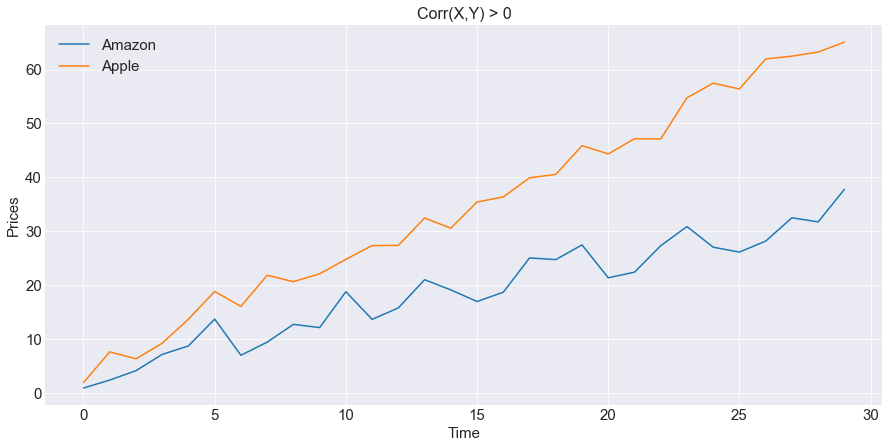
Imagine we have data from four stock prices:

Amazon,
Apple,
Walmart, and
Microsoft.

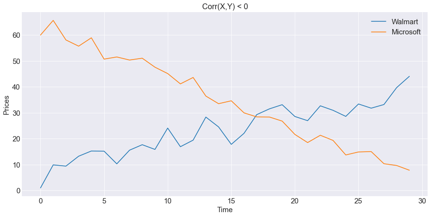
At the top, you have a graph in which you could see a positive Covariance: While Amazon stock price moves higher, Apple moves in the same positive direction. At the bottom, you can see that, when Microsoft moves down, Walmart does the opposite, moves higher, which means there is a negative Covariance between them.

Question: If variable A and B have a positive Covariance, then should we interpret that whenever variable A goes higher in value, B “always” goes in a higher value too?”

Not always. This direct or inverse comovement could also be strong or weak. If the positive or negative Covariance value is big, in absolute terms, then we say that the comovement is strong, if it is low, we say the comovement is weak.

What is a strong or weak comovement?

Well, what we can say is that a big positive Covariance, or a strong positive comovement, means that, most of the time, the two variables will move in the same positive direction.

The same for a negative Covariance: If we have a big negative Covariance value for two variables, in absolute terms, this means that we expect to see, most of the time, the two variables move in the opposite direction.

So, now with a clearer definition, you have a deduction and two more questions to test your knowledge:

Does Covariance measure the strong or weak relationship between two variables?
Can we have a perfect direct or inverse comovement between two variables?

For these questions, let us take you to our other important concept called Correlation.

What is Correlation?

You might have made a pause and taken a sip of your cup of coffee and might be saying to yourself: “Oh, here comes another definition, it’s a lot of information!”

Hey! Don’t worry at all! Correlation has, actually, a similar definition. Let’s put it formally first. Correlation measures the degree of the linear association between two variables.

We know, you are surprised, and ask: “Do we have the words ‘linear association”, again?”

Hey! Don’t hurry, we’re talking about this later. For now, we could say: While Covariance measures the direction of the comovement, Correlation not only measures that, but also the degree, or “strength”, of this relationship direction.

We’ll see later how this ‘strength’ looks like. For now, let’s express the differences between these two concepts below:

What are the differences between Covariance and Correlation?

Covariance	Correlation
Measures one thing	Measures two things
Infinite range	Finite range
It has unit of measurement	Free of unit of measurement
Scalable value	Non-scalable value

Difference #1: Covariance measures one thing and Correlation measures two things.

Covariance, as explained above, measures only the direction of the comovement of two variables. Correlation measures not only the direction of the relationship, but also the strength of this relationship.

So how well do Amazon and Apple stock prices move in the same or opposite direction?

You now have two technical tools to answer this question:

To find out whether two variables move in the same or opposite direction, you could use either the Covariance or the Correlation functions.
About “how well” this direct or inverse relationship is, you need to answer this with the latter.

Difference #2: Covariance and Correlation value range are not the same.

Covariance could have an infinite positive value or an infinite negative value, the range of values takes the whole real number spectrum. However, Correlation value range is only between -1 and +1.

So your question regarding a perfect comovement could be answered here: Since Covariance could have any real value, we could not appreciate with this statistical measure a perfect degree of linear association between two variables.

The best way to approach this question is with Correlation. If the Correlation of variables A and B has the value of +1, you can say without any doubt that both variables “always” move in the same direction. The same for a Correlation with a -1 value: you can say without any doubt that both variables “always” move in the opposite direction.

Here you can understand Difference #1. When the Correlation is between -1 and 1, the comovement is not perfectly negative or positive, respectively. Last but not least about this difference, we must say that it’s almost impossible to see real world variables having a Correlation exactly equal to +1 or -1.

Difference #3: Covariance and Correlation have different measure units.

You will get to understand it mathematically later. By now, we can say that Covariance has as a unit of measurement the multiplication of the two variables’ units of measurement.

For example, if you have two stock prices which are Amazon and Apple, which both have as unit of measurement the dollar, you will have for the Covariance a unit of measurement of: Dollar times Dollar, which is Dollar squared.

However, Correlation doesn’t have any unit of measurement at all. Don’t hurry to worry! Sip your coffee and wait a little bit more to fully understand this.

Difference #4: Covariance could change in value if the variables are scaled differently, Correlation is not affected by this.

Let us give you an example to understand this difference. You have two stock prices, Amazon and Apple, and then you calculate their Covariance and Correlation, which result in “a” and “b” respectively.

Next, you decide to multiply the two stock prices by 1000, and you calculate, again, their Covariance and Correlation, which result in values “c” and “d”. Something interesting that you will find is that:

Covariance “a” is different from Covariance “c” and,
Correlation “b” is equal to Correlation “d”.

When you scale one or both variables, Covariance will change in value accordingly. However, Correlation is not affected by the scale change.

How to Calculate Covariance and Correlation?

Up until now, we explained to you everything about their concepts and their properties. But from now on, you will have a better grasp with the mathematical formulas.

First, you must differentiate between what is a population and sample data. Once you are familiar with these two concepts, let’s begin with the presentation of the formulas:

We start with Covariance.

Population Covariance:

$$ \sigma_{X,Y}^{2} = \frac{\sum_{i=1}^{N}\Bigl(X_{i}-\overline{X}\Bigr)\Bigl(Y_{i}-\overline{Y}\Bigr)}{N} $$Where:
$ \sigma_{X,Y}^{2} $: Population Covariance between variables $X$ and $Y$.
$X_{i}$: The $i^{th}$ observation of the $X$ variable.
$\overline{X}$: The mean value of variable $X$.
$Y_{i}$: The $i^{th}$ observation of the $Y$ variable.
$\overline{Y}$: The mean value of variable $Y$.
$N$: Total number of observations for variable $X$ o $Y$.

Sample Covariance:

$$ S_{X,Y}^{2} = \frac{\sum_{i=1}^{N}\Bigl(X_{i}-\overline{X}\Bigr)\Bigl(Y_{i}-\overline{Y}\Bigr)}{N-1} $$Where:
$ S_{X,Y}^{2} $: Sample Covariance between variables $X$ and $Y$. The other variables are the same as for the Population Covariance

So, in simple words, how could we explain the Covariance formula? Let’s say it in this way: Covariance is a measure in which we multiply each deviation from the mean of X and Y, given by (Xi-X) and (Yi-Y) respectively, and then we sum all these products and divide them by N.

It resembles the formula of the Variance of a variable, right? Well, both formulas are almost similar, the only difference is that in the Variance formula you see the deviations from the mean squared, for the Covariance, you don’t see a squared deviation.

But the Variance formula can also be written as:

$$ \sigma_{X,Y}^{2} = \frac{\sum_{i=1}^{N}\Bigl(X_{i}-\overline{X}\Bigr)^2}{N}=\frac{\sum_{i=1}^{N}\Bigl(X_{i}-\overline{X}\Bigr)\Bigl(X_{i}-\overline{X}\Bigr)}{N} $$

So, you get it? Variance and Covariance formulas are actually identical; the difference resides in the second parenthesis, which is replaced by the deviations of a second variable. Variance refers to a single variable, Covariance refers to two variables, that is why it’s called “Co” Variance.

The sample Covariance is the same as the population variance, but instead of N, we divide the dividend by N-1. The explanation of this difference can be found in the “Standard deviation for sample data - Bessel's correction” section of this blog.

As you could guess, X is in X units, and Y is in Y units. So, the Covariance formula, since it is a multiplication of these two variables, will be in XY measure units.

Let’s go now for the Correlation formula:

$ \rho_{X,Y} = \frac{\sum_{i=1}^{N}\Bigl(X_{i}-\overline{X}\Bigr)\Bigl(Y_{i}-\overline{Y}\Bigr)}{\sqrt{\biggl(\sum_{i=1}^{N}\Bigl(X_{i}-\overline{X}\Bigr)^2\biggr)\biggl(\sum_{i=1}^{N}\Bigl(Y_{i}-\overline{Y}\Bigr)^2\biggr)}} = \frac{\sum_{i=1}^{N}\Bigl(X_{i}-\overline{X}\Bigr)\Bigl(Y_{i}-\overline{Y}\Bigr)}{\sqrt{\biggl(\sum_{i=1}^{N}\Bigl(X_{i}-\overline{X}\Bigr)^2\biggr)}\sqrt{\biggl(\sum_{i=1}^{N}\Bigl(Y_{i}-\overline{Y}\Bigr)^2\biggr)}}$$$ \rho_{X,Y} = \frac{Cov(X,Y)}{\sigma_X\:\sigma_Y} $$Where:
$ \rho_{X,Y} $: Correlation between variables $X$ and $Y$.
$Cov(X,Y)$: Covariance between $X$ and $Y$.
$\sigma_X$: Standard Deviation of variable $X$.
$\sigma_Y$: Standard Deviation of variable $Y$.

So, how could we explain this formula in simple words? Well, you already know the dividend, and about the divisor, if you could remember the Variance formula, you can realize that the divisor is the multiplication of the standard deviation of both variables X and Y.

So we can say that Correlation is the Covariance divided by the Standard Deviations of the two variables. You might be thinking that the Covariance and the Standard Deviation have as a divisor “N” or “N-1”, so you could think that we wrote the first formula wrongly.

Don’t worry, let us make you see what happened with the divisors:

$ \rho_{X,Y} = \frac{\frac{\sum_{i=1}^{N}\Bigl(X_{i}-\overline{X}\Bigr)\Bigl(Y_{i}-\overline{Y}\Bigr)}{N}}{\sqrt{\Biggl(\frac{\sum_{i=1}^{N}\Bigl(X_{i}-\overline{X}\Bigr)^2}{N}\Biggr)}\sqrt{\Biggl(\frac{\sum_{i=1}^{N}\Bigl(Y_{i}-\overline{Y}\Bigr)^2}{N}\Biggr)}} = \frac{\frac{\sum_{i=1}^{N}\Bigl(X_{i}-\overline{X}\Bigr)\Bigl(Y_{i}-\overline{Y}\Bigr)}{N}}{\sqrt{\biggl(\sum_{i=1}^{N}\Bigl(X_{i}-\overline{X}\Bigr)^2\biggr)\biggl(\sum_{i=1}^{N}\Bigl(Y_{i}-\overline{Y}\Bigr)^2\biggr)\Biggl(\frac{1}{N^2}\Biggr)}} $

$ \rho_{X,Y} = \frac{\sum_{i=1}^{N}\Bigl(X_{i}-\overline{X}\Bigr)\Bigl(Y_{i}-\overline{Y}\Bigr)\Biggl(\frac{1}{N}\Biggr)}{\sqrt{\biggl(\sum_{i=1}^{N}\Bigl(X_{i}-\overline{X}\Bigr)^2\biggr)\biggl(\sum_{i=1}^{N}\Bigl(Y_{i}-\overline{Y}\Bigr)^2\biggr)}\Biggl(\frac{1}{N}\Biggr)} = \frac{\sum_{i=1}^{N}\Bigl(X_{i}-\overline{X}\Bigr)\Bigl(Y_{i}-\overline{Y}\Bigr)}{\sqrt{\biggl(\sum_{i=1}^{N}\Bigl(X_{i}-\overline{X}\Bigr)^2\biggr)\biggl(\sum_{i=1}^{N}\Bigl(Y_{i}-\overline{Y}\Bigr)^2\biggr)}}\frac{\Biggl(\frac{1}{N}\Biggr)}{\Biggl(\frac{1}{N}\Biggr)} $

$ \rho_{X,Y} = \frac{\sum_{i=1}^{N}\Bigl(X_{i}-\overline{X}\Bigr)\Bigl(Y_{i}-\overline{Y}\Bigr)}{\sqrt{\Biggl(\sum_{i=1}^{N}\Bigl(X_{i}-\overline{X}\Bigr)^2\Biggr)}\sqrt{\Biggl(\sum_{i=1}^{N}\Bigl(Y_{i}-\overline{Y}\Bigr)^2\Biggr)}} $

$$ \rho_{X,Y} = \frac{Cov(X,Y)}{\sigma_X\:\sigma_Y} $$

Now you get it? The divisors from the Covariance and the Standard Deviations canceled each other. Besides, the dividend, as explained earlier, has as a measure unit the multiplication of both the measure units of X and Y. The divisor has as a measure unit, also, the multiplication of the measure units of both Standard Deviations, which are from X and Y.

Consequently, since the dividend and the divisor have the same XY measure unit, they cancel each other and you get the Correlation value free of a measure unit. Now you can understand the Difference #3 explained before, right?

Besides, you can now understand Difference #4. Why? Because the Covariance ends with a XY measure unit, so whenever you change the scale of any of the two variables, then you will scale, too, the divisor’s measure unit.

Meanwhile, since the Correlation formula does not have a measure unit, the change of scale you could make to, again, any of the two variables, won’t affect the Correlation range which is between -1 and 1.

We got through all these explanations and you might ask now about:

Importance of Covariance and Correlation

Well, you now ask this important question. The answer resides in the essence of Economics and Finance. Finance, as an essential part of Economics, is about markets where economic agents buy and sell assets from one or more markets.

Within markets or between markets, assets can move in the same or opposite direction with any other asset due to the same agents that make transactions everyday.

Asset prices change according to agent’s behaviors, market conditions, etc. If there’s a person who buys 100 shares of Apple or if there’s a crowd who sells their bank shares due to a bank run, every single person’s transaction has consequences not only on the asset itself, but also on other stocks or in other markets.

Markets are interrelated, so Correlation and Covariance are an essential part of the study of financial markets. If markets or financial assets weren’t interconnected, we wouldn't need to take care of comovements.

You now know not only what these two concepts mean but also why they are important. We get to our main purpose.

So, now, you want to trade, right?
You are ready to check the correlation of the Apple and Amazon stock prices and now you are prepared to press the BUY and SELL buttons in your broker’s platform to start investing. Aren’t you?

No! Wait a minute! Let us explain to you, before you make a decision, the real world applications of Covariance and Correlation in trading and investment.

Trading Applications of Covariance and Correlation

Trading Application #1: Portfolio Volatility Computation

When you start investing in more than one stock, you must consider how well the volatility of your portfolio is behaving. The computation of this Portfolio Volatility is only possible to be done once you fully understand both how Covariance and Correlation work.

So, please, don’t press the BUY button yet. You can check our course on Portfolio Management on Quantra to get to know more about it. Wait a bit more to let us explain to you more.

Trading Application #2: Statistical Arbitrage

Whenever you get into Statistical Arbitrage you have to understand the definitions of Correlation and Cointegration. Statistical Arbitrage does not make use of Correlation, but it’s really important to comprehend the difference between the two concepts.

Our course on Statistical Arbitrage Trading explains all about this. We can guess that you want now to start pressing the BUY and SELL buttons to do arbitrage, right? We told you, wait for more!

Trading Application #3: Correlated Variables in a Regression Estimation

One of the main conditions to make a regression between two or more variables is to have uncorrelated independent variables. So, since you already know the meaning of Correlation, you are now able to correct a problem in case there is a violation of this condition in your regression estimates. You can expand your knowledge about this topic with this course on Trading with Machine Learning: Regression.

Trading Application #4: Correlation to Predict Asset Prices

See, financial asset prices, contrary to what happens to variables in a controlled physics experiment, tend to suffer regime changes across time. So in case you calculate the Correlation of a US Treasury 2-year Bond Yield with the FED Funds Rate using data from 2021, this value won’t necessarily be the same for the year 2022.

Correlation through time could vary greatly and this mostly happens in adverse economic shocks or economic or financial crises. Be careful while using Correlation to predict your next signal to trade!

Trading Application #5: ARMA Models to Predict Asset Price Returns

So, have you heard about Autoregressive Moving Average (ARMA) Models? This model tries to forecast asset price returns with their past returns estimates calculated through a regression model, in which the moving average of the regression errors is also important.

Here you will get to know what AutoCovariance and AutoCorrelation functions are. So in order to understand these two concepts, you have first to understand the two concepts of this article.

What does an autocorrelation function look like?

Well, remember that the Correlation function is calculated based on two variables and remember also that the ARMA models try to predict asset price returns with their previous returns. So if you say these returns could be called rt, then, the autocorrelation function can be expressed as:

$$ \rho_{r_{t},r_{(t-1)}} = \frac{Cov(r_{t},r_{(t-1)})}{\sigma_{r_{t}}\:\sigma_{r_{(t-1)}}} $$

Do you want to know more? Get access to this amazing course on Time Series Analysis in Quantra.

Trading Application #6: Causality and Correlation Are Not the Same Thing

This is more of a trading knowledge so pay attention to this. Causation means that a movement in Apple Stock price causes a movement in Amazon Stock price. But, what do we mean by “causes” here? Well, Causation is even discussed philosophically in Economics. The philosophical discussion hasn’t ended up to now. Let me give you an example so you could understand it better.

Imagine we have the number of litres of rainwater that falls each month in New York City and we also have the monthly GDP of New York city as well. You calculate the Correlation between them and get a value of 0.95.

You get to say: “Oh, that’s interesting! I can say, then, that, whenever it’s raining a lot in the city, this will cause the NY GDP to increase.” No! You can’t say that a lot of rainwater ‘causes’ an increase in GDP; or vice versa, that an increase in GDP ‘will cause’ an increase in rainwater in the city.

Correlation simply means that you could find a pattern of comovement between these two variables but it doesn’t mean that there is an economic causation between rainwater and GDP.

So, whenever you are talking, as a trader, about Correlation, you must always keep in mind that this concept is not necessarily the same as Causation. Putting it in another way:

Causation always implies Correlation, but Correlation doesn’t always imply Causation.

Trading Application #7: Correlation Stylized Facts

This is also important information to incorporate into your background knowledge. Some worldwide correlations are important to consider when you want to trade in some financial assets.

Here we present you some stylized facts to keep in mind whenever you want to trade with these assets:

Crude Oil and Currencies: Crude-oil net exporters like Russia, Canada, Venezuela or Saudi Arabia see their currencies fall whenever the crude oil price falls. However, crude net importers like Japan tend to see their currency appreciate whenever the crude oil price falls.
Flight-to-Quality: Whenever there is a financial turmoil in an important country or part of the world, like the 1997 Asian financial crisis, investors tend to get their money out of these high-yield countries and buy US Treasury bonds. This action makes the affected countries’ currencies depreciate highly against the dollar and the US Treasury bonds tend to soar in value. Consequently, in the Asian crisis, there was a negative correlation between the asian countries’ currencies and the US bond prices.
Equity-Bond Negative Correlation: For example, whenever the US economy starts to boom, investors reallocate their portfolios. They invest heavily in more risky assets and less in Treasury bonds. When the economy enters a recession, it happens the opposite, there’s a greater investment in fixed income and less in equity securities. This negative correlation between Equity and Bonds is a common feature of countries around the world.
Gold Time-Varying Correlation: When world investors are more prone to invest in risky assets, there is an increase in the positive correlation between gold and the US stock market. When they become more risk averse, due to a global recession, gold becomes inversely correlated with the US stock market.
Gold and Inflation: When world inflation goes up, investors tend to increase their portfolio allocation to gold, meaning, the correlation between gold and inflation is positive. Gold behaves as a hedge against inflation. The precious metal maintains your buying power when inflation rises above expectations.
Gold and US interest rates: When the US sees its interest rates go up, then this means the economy is in good strength. This makes world investors allocate their resources to more risky assets. Thus, gold starts to decline in value in this period. We can say Gold and US interest rates have a negative correlation throughout time.
Geopolitics and Gold: Whenever there are adverse geopolitical shocks that affect the whole world, gold price tends to increase, since this precious metal acts as a ‘safe haven’.
Returns-Volatility Correlation: When stock prices fall, companies suffer an increase in their debt-to-equity ratio, which in turn, makes its stock price return volatility increase. This negative correlation between stock price returns and its volatility is called “the leverage effect”. When you trade with stocks and want to model volatility, you should consider this effect on your estimation in order to capture the negative correlation.

Covariance and Correlation Simple Exercise Examples

How to Calculate Covariance?

You are now ready for this, right? Ok, let’s start with a simple example. Imagine we have two asset prices called Microsoft and Tesla, and we have 5 days of data for each stock.

Below we have the data as a table presented below:

Date \ Stock	Microsoft	Tesla
Day 1	240	850
Day 2	265	800
Day 3	255	820
Day 4	280	870
Day 5	301	900

Since we have a sample instead of a population data, we will use the sample Covariance and the Correlation function. First of all, we know that we have 5 observations, that’s why our N variable is 5.

Then, we have to calculate the mean for each Stock. We’ll help you with that, these two means are: 268.2 and 848 for Microsoft and Tesla, respectively. Next, we have to calculate the deviations of each observation from the mean, this must be done for each stock:

Date \ Stock	Microsoft	Tesla	Microsoft Deviations from the Mean	Tesla Deviations from the Mean
Day 1	240	850	-28.2	2
Day 2	265	800	-3.2	-48
Day 3	255	820	-13.2	-28
Day 4	280	870	11.8	22
Day 5	301	900	32.8	52

Once you are done with that, you can proceed to multiply both deviations for each date and then sum all the multiplications to get the dividend of the Covariance Formula:

Microsoft’s Deviations from the Mean	Tesla’s Deviations from the Mean	Multiplication of both Deviations
-28.2	2	-56.2
-3.2	-48	153.6
-13.2	-28	369.6
11.8	22	259.6
32.8	52	1705.6
	Covariance Dividend	2432

What’s missing to calculate Covariance?

You’re almost done. You have the dividend, you’re missing the divisor. The divisor is just the total number of observations minus one. So let’s divide the Covariance Dividend with (N - 1):

$ Cov(Microsoft,Tesla) = \frac{2432}{5-1} = \frac{2432}{4} $
$ Cov(Microsoft,Tesla) = 608 $

Remember the definition? Covariance measures the direction of the comovement, in this case, between Microsoft and Tesla. So what interpretation can we get from this value? Well, we can say that, since 608 is a positive number, we conclude that there is a positive comovement between these two stock prices.

Now you ask me, How “strong” is this comovement between Microsoft and Tesla? That could be answered with the Correlation coefficient.

How to Calculate the Correlation coefficient?

Once we have the Covariance value, you can remember from above, we only need the Standard Deviations from both Microsoft and Tesla. We are going to help you with those values. The Standard Deviation of both Microsoft and Tesla are 23.42 and 39.62, respectively. So applying the formula, we get:

$ Cov(Microsoft,Tesla) = \frac{2432}{23.42*39.62} = \frac{2432}{928.15} $
$ Cov(Microsoft,Tesla) = 0.66 $

If we choose 0.5 as our threshold to decide if a correlation value is close to 1 or close to zero, that depends on the researcher, and since 0.66 is greater than 0.5, we could say that the comovement between Microsoft and Tesla is positive and also strong.

What did we mean by “degree of linear association” in the Correlation definition?

Way before, we explained to you that Correlation measures the degree of the linear association between two variables. This explanation is the formal definition you will find in textbooks of Statistics.

How could you face this explanation with a simple understanding?
Let’s do that now.

We know that Correlation has a value range between -1 and +1. It could also be zero, right? Let’s graph those two extreme cases and a close-to-zero one in a scatter plot:

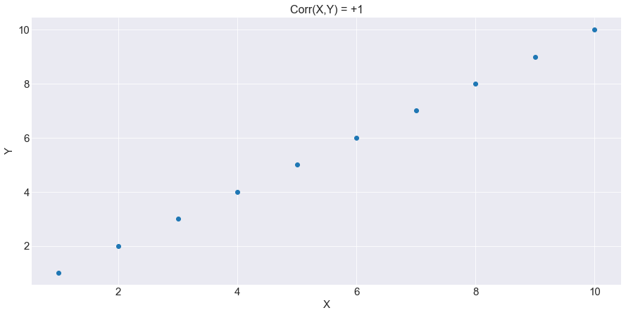
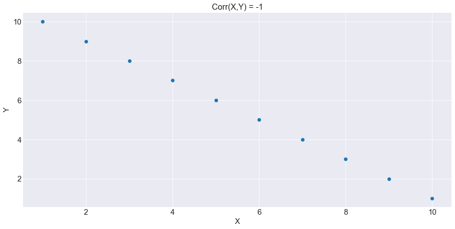
As you can see, when Correlation is perfectly +1 or -1, the scatter plot forms itself like a line. That means both variables A and B have a linear relationship or linear association.

If the Correlation is close to one, you could say that, if you graph a line throughout the values, you will have this line with a positive slope. If the Correlation is close to -1, and if you graph a line throughout the values, you will have a line with a negative slope. As the value decreases from 1 to zero, this linear association becomes less clear, the same as the value increases from -1 to zero.

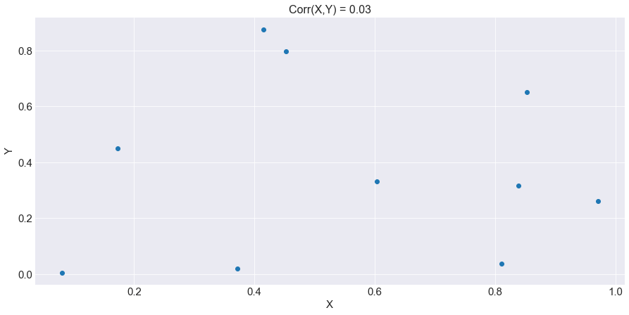
Correlation equal to zero or very close to zero means that there is no correlation at all between the two variables and you will also see for this Correlation value almost a random scatter plot.

Using our correlation definition from above, the strength of a positive correlation can be understood as the formula value tending from zero to +1. The strength of a negative correlation can be understood as the formula value tending from zero to -1.

Let’s see graphically how weak or strong correlations behave:

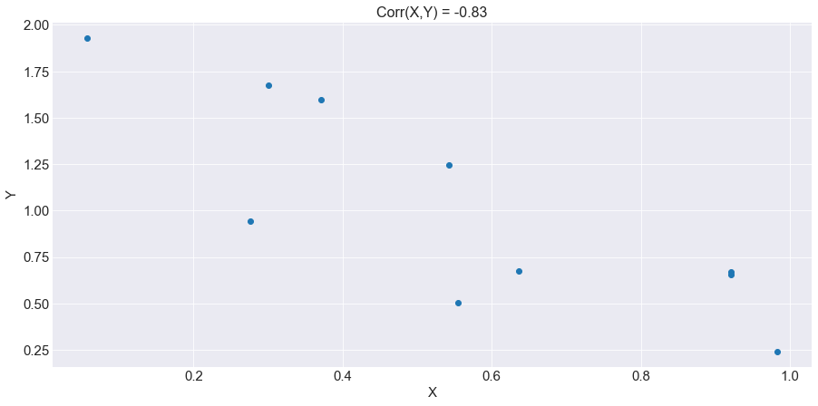
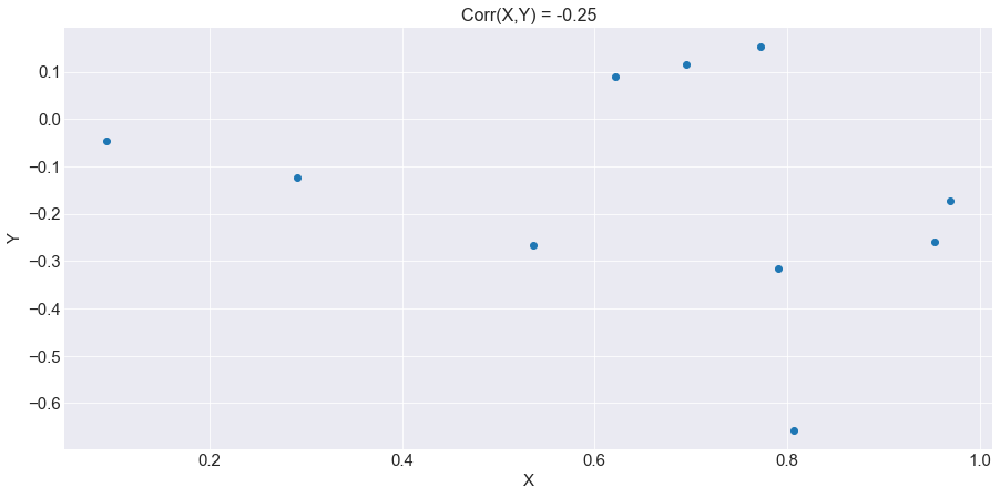
You already saw what a perfectly negative Correlation looks like. Now you can see from the above graphs what strong and weak correlations might look like. The top graph shows a negative Correlation of -0.83 and the bottom graph shows a Correlation equal to -0.25.

As you can see, when the value gets close to -1, you can say that this negative Correlation is strong. However, as the Correlation approaches zero, the linear association can’t be seen clearly in the graph, and we also say that this negative correlation is weak.

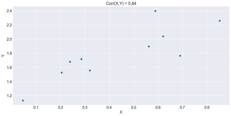
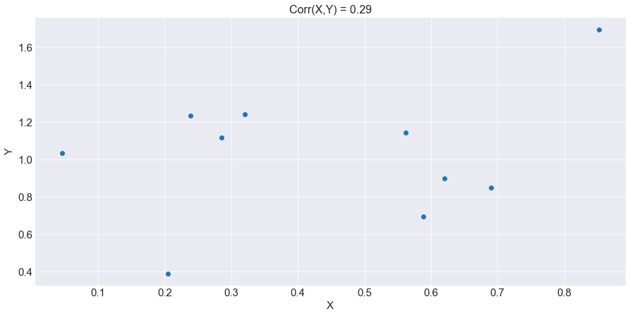
Next, let’s see the case for positive Correlations. The top graph shows a positive Correlation of 0.84 and the bottom graph shows a Correlation equal to 0.29. As you can see, when the value gets close to 1, you can say that this positive Correlation is strong.

However, as the Correlation approaches zero, the linear association can’t be seen clearly in the graph, and we also say that this positive Correlation is weak.

We showed above a graph with a zero Correlation case. Now, you could ask us maybe, isn’t there any other form of no correlation?

Let’s see this other graph:

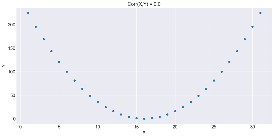
As you can see, this Correlation between X and Y is zero, it has both a positive and negative linear association at the same time. So there are two types of graphs regarding a Correlation equal to zero:

A random scatter plot, and
A non-linear scatter plot.

What are good Covariance and Correlation values?

Seeing the last graphs or even before, you might have asked yourself this question. You must know the answer so we’ll explain it here. Actually, there is no “good” or “perfect” value for a Covariance and Correlations function for all cases.

For example, for portfolio management, it’s a good value for the Stock Covariances to be negative, so you can have a better diversification between assets. For the independent variables in a regression estimation, you consider a good value for their Correlations to be close to zero.

For an ARMA model, you will want to have the autocorrelation functions be different from zero, in order to confirm that the construction of the model is appropriate for the stock price returns.

As you could see, a good value for our Covariance or Correlation formulas depends on what you’re looking for: It depends on the trader or the researcher, and also on the topic you are talking about.

Covariance and Correlation Computation Examples in Python

Now let’s make use of real-world data to compute these two important concepts in our main programming language called Python:

How to Calculate Covariance and Correlation in Python

Let’s download Microsoft and Tesla Stock prices to use them for our calculations:

We first set up the environment to get things done. Don’t forget to install the ‘yfinance’ library in case you don’t have it:

Then we get daily historical data with the ‘yfinance’ API. We will download data from the year 2021 up until March 3, 2022. We also adjust the OHLC and Volume values, with their corresponding Adjusted Close, setting to True to the auto_adjust condition.

Next, we calculate the Covariance and Correlation for the whole sample period:

Here's the output:

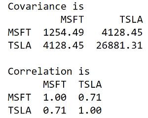
Here we have to explain something about this output. As you can see, both for the Covariance and Correlation there is a table for each one.

The special tables you see are actually a Covariance Matrix for the above matrix and the Correlation matrix for the below matrix. You will have in the Covariance matrix diagonal the Variances, which are 1312.74 and 26796.55 for Microsoft and Tesla respectively. The matrix lower triangular should be a mirror of the upper triangular, meaning it should have the same values.

The same for the Correlation matrix shown below. The Correlation matrix diagonal represents the Correlation function applied not with another variable, but with the same one. We mean, for the Matrix(1,1), it is a correlation function applied with the Microsoft Stock Price against the same Stock Price, Corr(Microsoft,Microsoft).

You can prove that we leave you this as an exercise when you apply a Correlation function only with one Stock price, you will always get +1 as value. These Covariance and Correlation matrices could be deployed for more than two variables too, and they will follow the same properties as per the lines above explained.

Once you understand what we just explained, we can go to our final Covariance and Correlation computations:

How to Calculate the Rolling Covariances and Correlations in Python.

As we explained before, Correlation and Covariance could change in value as time passes. That’s why it’s essential to calculate Correlation or Covariance throughout time. One way to do this is by calculating the rolling Covariances and Correlations for our Microsoft and Tesla Stock Prices.

We mean rolling here in the sense that, specifying first a number of days called “n”, you will get both the Covariance and the Correlation functions applied for each day with “n” previous days as the history data window to estimate them.

It’s super simple. Just pay attention to the following. Since you know that the pandas properties called “.cov” and “.corr” get you a matrix, you might guess that if you applied a rolling Covariance and Correlation functions you will also get a matrix for each day.

In order to avoid getting the whole matrix for each day, you extend each property called by unstacking them and, then, calling, for both functions, the Covariance and Correlation functions between MSFT and TSLA only. We want to set as the historical data for each observation a 20-day window to calculate the functions, a monthly window. See below:

Here's the output:

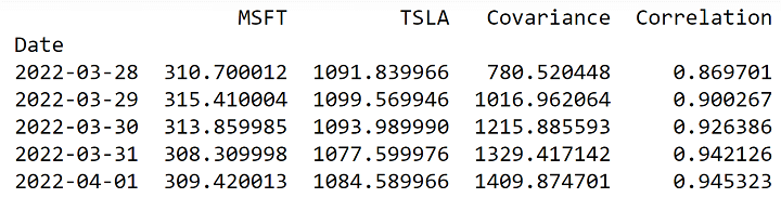
Now let’s see graphically how Covariance and Correlation look throughout time:

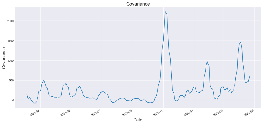
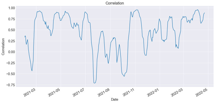
As we told you before, you can see that both Covariance and Correlation change throughout time. There are some periods where Microsoft and Tesla move in the same direction, while there are other periods where they move in the opposite direction.

Be careful and be patient when trading! Risk management is something valuable in order to trade well in the financial markets!

Conclusion

Now, you have a better understanding of what these two concepts mean. This article also made you knowledgeable about the intricacies of the formulas. You not only know that but also comprehend how to apply Covariance or Correlation in Trading.

You are almost there to press the BUY button. It’s time now to start learning strategies in which you can potentially use these two concepts without any problem.

So, do you want to start trading with more than one asset and use the Correlation and Covariance formulas? Why not? You can enroll into our course Quantitative Portfolio Management so you could start using these concepts now!

Are you ready? Go Algo!

Disclaimer: All investments and trading in the stock market involve risk. Any decision to place trades in the financial markets, including trading in stock or options or other financial instruments is a personal decision that should only be made after thorough research, including a personal risk and financial assessment and the engagement of professional assistance to the extent you believe necessary. The trading strategies or related information mentioned in this article is for informational purposes only.

Advanced Momentum Trading: Machine Learning Strategies Course