
Is it possible to use Probability in Trading? How can someone do so? This comprehensive guide provides you an in depth knowledge of the concept of Probability and it's application in trading. With various examples, it discusses probability and explains why you need to have a good idea about how it works.
This article is divided into the following sections:
What is probability?
Probability is the study of events and outcomes that involve an element of uncertainty. Tossing a coin for example involves uncertainty, as does investing in the stock market.
Probability is a tool that you can use to deal with this uncertainty and make better investment decisions. There are considerable amounts of fluctuations in the stock prices post-earnings announcement.
Wouldn’t it be better if you knew the probability of an increase or decrease in the price of the stock?
You could make a better decision and the chances of you making a profit out of that trade increase as well.
For example, the probability of Snapchat stock rising post-earnings announcement is 80% and fall is 20%. So, if you buy the stock, there is an 80% probability that you will make a profit and a 20% probability that you will make a loss. With this information, you will be more confident to buy the stock as you have the odds in your favour.
Now that we understand what probability is, and how it can help you to make better decisions. How do you calculate this probability?
Probability formula
You ask 100 analysts to take a poll on their analysis of Snapchat’s stock price movement.
- 80 out of the 100 analysts believed that the price will increase and 20 believed that the price will decrease.
- So, if A is an event that the stock price increases, the probability of event A is 80/100, i.e., 0.8 or 80%.
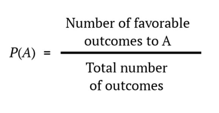
The probability of any event A is calculated by this formula:
Application of Probability
When you think of the application of probability, what is the first thing that comes to your mind? It is probable that flipping a coin or rolling a dice may be your first thought. Let’s not limit ourselves to these events only.
Some events will always happen as the sun rises in the east and sets in the west. There is a 100% probability of this happening daily or we can say that this is a certain event.
What if uncertainty comes into the picture?
Let’s say you want to bet on which team will win the next match between Barcelona and Real Madrid.
- Since both are strong teams, you’re unsure of which team to bet on
- You have been presented with the information that the match will be held in Barcelona’s home stadium
- There is a higher chance of Barcelona winning a home match.
Now, which team will you bet on? Probably Barcelona if you’re not biased towards any team. This is one instance where you can use probability to make better decisions.
Two properties of probability
When you have calculated the probability of any event, you must make sure the calculated probability satisfies two properties, which together constitute its definition:
a) The probability of any event A is a number between 0 and 1, i.e., 0 ≤ P(A) ≤ 1.
0 indicates an impossible event such as rolling 7 on a six-sided die and 1 indicates that the event will certainly happen such as the sun rises in the east.
b) The sum of the probabilities of any set of mutually exclusive and exhaustive events equals 1.
You may be wondering, what are mutually exclusive and exhaustive events?
Let’s take an example of a price change in the Tesla stock after a change in the market sentiment affected by tweets. There are three possible outcomes at a point in time. Either the price will increase, decrease, or will remain the same, and these events cannot happen at the same time.
Such events are called mutually exclusive events. When all the possible outcomes are covered and you’re not missing out on the possibility of the occurrence of any event, then such events are called exhaustive events.
So, if the probability of an increase in the price was 0.9 or 90%, the probability of a decrease in the price was 0.06 or 6% and the probability that the price will stay the same was 0.04 or 4% then you can observe that the probabilities lie between 0 and 1 and sum of all the probabilities equals 1.
Types of probability
Now that we understand what probability is and how it is calculated, let's delve into the different types of probabilities. It is important to understand this as it can assist you in making your own decisions.
Probability can be broadly classified into two categories:
- Subjective Probability
- Objective Probability
Subjective probability
Subjective probability is a type of probability that draws on personal or subjective judgment. It varies from person to person.
For example, during the 2008 financial crisis, not a lot of people bet against the housing market. But the ones who did, made extraordinary profits from it while economies all around the globe suffered.
The opinions of people who predicted the crash were subjective and the probability of occurrence of this event was different for everyone.
Objective probability
Objective probability on the other hand does not vary from person to person. It can be calculated by experiments and observation.
One of the most common ways to estimate the probability of an event is by analysing the historical data because we tend to believe what has happened in the past will continue to happen in the future.
Let’s understand this with the help of a hypothetical scenario for Apple stock.
You have observed that the Apple stock price increases post the launch of the new iPhone every year. Therefore, there is a high probability that the price will increase this year as well.
This is known as an objective probability because it was deduced through historical analysis and observation rather than your personal biases and opinions.
Deducing the probability of events with only a few possible outcomes seems pretty easy, right? But what if an event had 100 possible outcomes?
In that case, it becomes hard to draw any inferences and apply them in real-life events to make substantial decisions.
Probability distributions solve that problem. As experiments and scenarios become more complex, using distributions is an effective solution.
What is a probability distribution?
A probability distribution is a statistical function that describes all the possible values and likelihoods that a random variable can take within a given range.
Let’s break down this definition with an example. You want to record the daily returns of Amazon stock for 100 days. Here, the random variable is the daily returns. The range varies from 0 to 100 days.
You record the returns in a tabular format. Through the distribution, you can analyse the average returns of the stock and how dispersed the returns are from the average return. It is useful when you want to know all the possible outcomes and which outcome is most likely to happen.
Statistically, we denote the random variable like x, and the likelihood that this random variable takes a specific value of x is denoted by p(x).
You need to know the type of random variable so that you can analyse your data set better. The type of a random variable determines the probability distribution.
There are two types of random variables:
- Discrete random variables
- Continuous random variables
Let’s understand the probability distribution for each type:
Discrete probability distribution for discrete random variables
When you toss a coin or when you take a trading decision to buy, sell or hold a stock, your answer is a discrete value. These two are examples of a discrete distribution because there are no in-between values.
Let’s say you want to calculate the probability of the market rising or falling for two consecutive days, assuming an equal probability of the market rising or falling each day. We will ignore the possibility of no change for the sake of simplicity.
You will get the following set of outcomes. Here, “R” denotes Rising and “F” denotes Falling.
|
Outcome |
Possible Combinations |
Probability |
|
1 Rise |
RR | ¼ = 0.25 |
|
1 Rise, 1 Falls |
RF or FR | ½ = 0.5 |
|
2 Fall |
FF | ¼ = 0.25 |
We have four possible outcomes. The market rises for 2 consecutive days, which is one out of the four possible outcomes. Therefore, the probability of this event is ¼ or 0.25. Similarly, we can calculate the probability of the market falling for two consecutive days.
The next possible set outcome is that the market falls on the first day and rises the next day or vice versa. This creates two possible outcomes. The probability of this event is 2/4 or 0.5.
Therefore, for this event, the discrete values create a discrete probability distribution.
Probability distribution for continuous random variables
When there is a change in the returns of a stock within a particular range, there are an infinite number of other valid values between two values. This is because accurate measurements can go up to any decimal value. The returns of a stock, for example, is a continuous random variable.
Normal distribution using Python
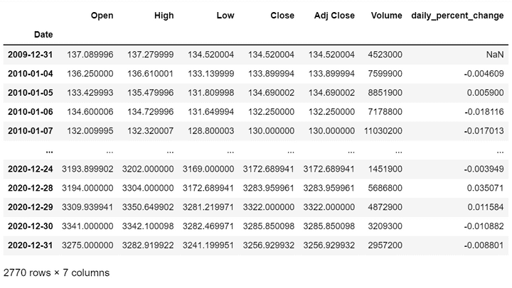
Let’s take amazon stock for example. You can download historical data from Yahoo Finance. For our dataset, we will use the following code in python.
This will give the time-series data set for Amazon. We calculate the daily percentage change for the adjusted close price of the stock and store it in the data set under daily_percentage_change.
We’ll base our analysis on the daily percentage change in the price for this stock.
We get the following output:
Before plotting these values, we can calculate the mean percentage change and the standard deviation of the percentage change. Calculating these statistical measures helps us understand and analyse our data set better.
We get the following output:
Mean = 0.00135
Standard Deviation = 0.01999
The mean percentage change for the amazon stock is approximately 0.00135 or 0.135% and the standard deviation for the stock is approximately 0.01999 or 1.999%. The standard deviation tells us how far the value deviates from the mean. So, the major part of our data lies between mean ± standard deviation, i.e., 0.00135 ± 0.01999
Now, let’s plot our data.
We get the following output:
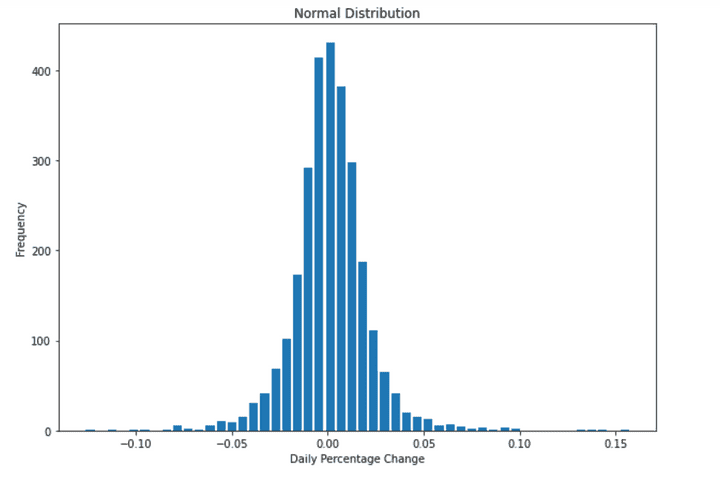
As you can observe, our distribution looks like a bell-shaped curve. This type of distribution is known as a normal distribution. It is a symmetric distribution with two parameters: mean and standard deviation.
The majority of data lies in the middle and the mean divides the data in half. The mean can be interpreted as the expected percentage change for the stock and the standard deviation as the risk associated with investing in this stock.
As the returns are normally distributed for this data set, we can calculate the minimum and maximum values or the range for the returns. This makes the improbable a bit more probable.
Conclusion
Probability is a mathematical concept that can be used and applied in the domain of trading. All smart traders and legendary investors like Warren Buffet use probability to create intelligent and well-designed trading strategies and refine decision-making.
In this blog, we discussed the basics of probability and the application of probability in trading with the help of Python.
You too can get started with algorithmic trading right from the basics of what, how, why, algorithmic trading strategies and regulations for setting up an algorithmic trading business, and much more in this Quantra course. Enroll now.
Disclaimer: All investments and trading in the stock market involve risk. Any decision to place trades in the financial markets, including trading in stock or options or other financial instruments is a personal decision that should only be made after thorough research, including a personal risk and financial assessment and the engagement of professional assistance to the extent you believe necessary. The trading strategies or related information mentioned in this article is for informational purposes only.
