A comprehensive guide to Dijkstra algorithm

The Dijkstra algorithm is a fundamental and widely used graph algorithm that finds the shortest paths between nodes in a graph. In this blog, we'll take a comprehensive look at the Dijkstra algorithm, starting with a clear explanation of what it is and how it works. We will then delve into its pseudo code, discuss a detailed example with a Dijkstra algorithm table, and analyse its time complexity.

Additionally, we'll discuss practical scenarios where the Dijkstra algorithm is most useful, and compare it with other notable algorithms such as Kruskal's and Prim's. By the end of this guide, you will have a clear understanding of how to find the shortest path in a graph using Dijkstra's algorithm and why it falls short when dealing with negative weights. So, let's embark on this journey to explore the Dijkstra algorithm and its intriguing world of shortest paths!

Here’s what we'll cover:

What is the Dijkstra algorithm?
How does the Dijkstra algorithm work?
Pseudo code of Dijkstra algorithm
Dijkstra algorithm table
Dijkstra algorithm time complexity
When to use the Dijkstra algorithm?
Dijkstra algorithm vs Kruskal algorithm
Dijkstra algorithm vs Prim algorithm
Prim algorithm vs Kruskal algorithm
How to find the shortest path using the Dijkstra algorithm?
Why does the Dijkstra algorithm fail for negative weights?

What is the Dijkstra algorithm?

The Dijkstra algorithm solves the shortest path problem for a graph with non-negative edge weights. It is known to be a greedy algorithm, which means it makes a series of choices that seem the best at the moment without thinking about future consequences.

Edsger W. Dijkstra (1930-2002) was an eminent physicist who made great advances in the world of distributed and concurrent computing and other fields of mathematics. The algorithm that bears his name finds the optimal solution to obtain the shortest path in a graph or net, although as we will see below there are improvements to the algorithm to enhance efficiency.

Greedy algorithms are typically used to solve optimisation problems, such as selecting the shortest path or the best order to execute tasks on a computer. In this context, the greedy algorithm selects the most promising segment or task at a given instant, without ever reconsidering whether that was the best decision later on. It is therefore a simple algorithm to implement since there is no need to control alternatives and no follow-up to undo previous decisions.

Properties of Greedy algorithms

Greedy algorithms such as Dijkstra algorithm, Kruskal algorithm or Prim algorithm are characterised by the following general properties:

Algorithms require solving a problem in an optimal way, where to construct the solution we have a set or list of candidates such as the edges of a graph, the tasks to plan, etc.
As the algorithm progresses, two sets are accumulated, one containing the candidates that have been evaluated and selected and the other containing the candidates that have been evaluated but rejected.
There is a function that checks whether a set of candidates form a solution to the problem, ignoring for the moment whether this is the optimal solution.
There is a second function that tests whether a given set of candidates is feasible, i.e. whether it is possible to reach a solution with other candidates to achieve the final solution. Again, it is ignored for the moment whether the solution is optimal.
There is a third function that selects the candidate that has neither been selected nor rejected and is the most promising candidate for the solution at a given point in time.
Finally, there is a fourth function called objective that returns the solution we have found, although it is strictly speaking not part of the greedy algorithm.

To solve the problem, we look for the set of candidates (first) that constitutes a solution and (second) that optimises the value of the objective function. The greedy algorithms proceed step by step.

Initially, the set of selected candidates is empty and at each step, the best candidate is considered to be added to this set by the selection function.

If the new extended set of selected candidates is not feasible for a solution, optimal or not, the candidate is rejected.
If the extended set of candidates still forms a possible solution, optimal or not, the new candidate is added to the set of selected candidates.

In this way, we continue to advance step by step until we find a solution that must necessarily be optimal. As we have said, these characteristics are common to the greedy algorithms although, as we will see later, the Dijkstra, Kruskal and Prim greedy algorithms have distinctive characteristics.

How does the Dijkstra algorithm work?

The Dijkstra algorithm solves the minimum path problem for a given graph. Given a directed graph G = {N, E} where N is the set of nodes of G and E is the set of directed edges, each edge has a non-negative length, we can talk about weight or cost too, and one of the nodes is taken as the origin-node.

The problem is to determine the length of the minimum path from the origin to each of the other nodes. As we have seen in the general characteristics of greedy algorithms, the Dijkstra algorithm uses two sets of nodes S and C. The set S holds the set of selected nodes and the distance to the origin node of each node at a given time. The set C contains all candidate nodes that have not been selected and whose distance is not yet known.

From this, we derive an invariant property N = S U C.
That is, the set of nodes is equal to the union of the sets of selected nodes and unselected nodes.

In the first step of the algorithm, the set S has only the node-origin and when the algorithm finishes it contains all the graph nodes with the cost of each edge.
We talk about a special node if all the nodes involved in the path from the origin to it are within the set of selected nodes S.
Dijkstra algorithm maintains a matrix D that is updated at each step with the lengths or weights of the shortest special path of each node of the set S.
When a new 'v' node is tried to be added to S, the shortest special path to 'v' is also the shortest path to all other nodes (see demonstration in the reference book).
When the algorithm is finished, all the nodes are in S and the matrix D contains all the special paths from the origin to any of the other nodes in the graph and thus the solution to our minimum path problem.

Let's see how the Dijkstra algorithm works in pseudocode before looking at the Python implementation.

Pseudocode of Dijkstra algorithm

The pseudocode of the Dijkstra algorithm outlines a method for finding the shortest paths from a starting node to all other nodes in a weighted graph.

Here's a concise explanation of the pseudocode of Dijkstra algorithm:
The function Dijkstra(L[1..n, 1..n]) initialises a matrix D[2..n] to store the shortest path distances and a set C of all nodes except the starting node. Initially, distances from the starting node to others are set based on direct edge weights from L.

The algorithm iteratively selects the node v in C with the minimum distance in D, moves v from C to the implicitly defined set S of nodes with determined shortest paths, and updates distances for the remaining nodes in C. For each node w in C, D[w] is updated to the minimum of its current value and the distance through v. This process repeats until all nodes are processed, and the matrix D is returned with the shortest path distances from the starting node.

The pseudocode of the Dijkstra algorithm is:

Dijkstra algorithm table

The Dijkstra algorithm table is used to illustrate the step-by-step process of finding the shortest path from a starting node to all other nodes in a weighted graph. This table provides a clear visualisation of how the algorithm updates distances and processes nodes iteratively.

Here's a breakdown of what each column in the table represents:

Step: This column is for the current iteration or step of the algorithm.
v: The v is the node selected in the current step that has the minimum distance and is moved from the set C to the set S.
C: This is the column for set of nodes that have not yet been processed (nodes remaining).
D: The column with D is the array of shortest path distances from the starting node to each node.

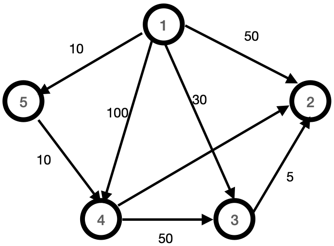
Assume the following routed graph:

Step	v	C	D
Initialization	-	{2, 3, 4, 5}	[50, 30, 100, 10]
1	5	{2, 3, 4}	[50, 30, 20, 10]
2	4	{2, 3}	[40, 30, 20, 10]
3	3	{2}	[35, 30, 20, 10]

The matrix D would not change if we did one more interaction to remove the last element of C {2} and for this reason, the main loop only repeats n-2 times..

Interpreting the Table

Let us understand the table with the interpretation below.

Initialisation:
C contains all nodes except the starting node (node 1).
D is initialised with the direct distances from the starting node to each other node.

Step 1:

Node 5 is selected (v = 5) because it has the minimum distance in D (distance = 10).
Node 5 is removed from C.
Distances are updated, and D is now [50, 30, 20, 10].

Step 2:

Node 4 is selected (v = 4) because it now has the minimum distance (distance = 20).
Node 4 is removed from C.
Distances are updated again, resulting in D being [40, 30, 20, 10].

Step 3:

Node 3 is selected (v = 3) with the minimum distance (distance = 30).
Node 3 is removed from C.
Distances are updated, resulting in D being [35, 30, 20, 10].

Final Note:

The matrix D would not change if the algorithm continued to remove the last element of C (node 2), which is why the main loop only repeats n-2 times.

Dijkstra algorithm time complexity

The time complexity of the Dijkstra algorithm depends on the data structures used. The time complexity of an algorithm, such as Dijkstra's, refers to the measure of the amount of time taken by an algorithm to complete as a function of the length of its input. In other words, it quantifies how the algorithm's runtime grows with respect to the size of the input data.

The initialisation requires a matrix L[1..n, 1..n] and therefore requires a time that is in the Order of n O(n).

The repeat loop requires looping through all the elements of C, so the total time is in the order of \(n^2. O(n^2)\)

The loop for each requires looping through all the elements of C, so the total time is on the order of \(n^2. O(n^2)\)

Therefore, the simple implementation of the Dijkstra algorithm requires a runtime that is \(O(n^2)\)

Depending on the implementation of the algorithm and as long as the number of edges is much smaller than \(n^2\), we can improve the complexity up to O((a + n) log n) if the graph is connected and is in O(a log n), but if the graph is dense we can only reach \(O(n^2 / log n).\)

To improve Dijkstra's simple algorithm, one can make an implementation of k-ary heaps as proposed by Johnson. Fredman and Tarjan further improve the complexity by using a Fibonacci heap. Also, the space complexity of the Dijkstra algorithm is O (V), where V is the number of vertices, due to the storage requirements for the distance and predecessor arrays.

See references for more information.

When to use the Dijkstra algorithm?

As we have seen, the Dijkstra Algorithm is used to solve the problem of minimum paths in a directed graph. The implementation we have been analysing always gives us the optimal matrix of minimum paths.

Typical applications of the Dijkstra algorithm:

Robot navigation.
Typesetting in TeX.
Urban traffic planning.
Tramp steamer problem.
Optimal pipelining of VLSI chip.
Telemarketer operator scheduling.
Subroutine in higher level algorithms.
Routing of telecommunications messages.
Approximating piecewise linear functions.
Exploiting arbitrage opportunities in currency exchange.
Open Shortest Path First (OSPF) routing protocol for IP.
Optimal truck routing through a given traffic congestion pattern.

Graphs

Graph	Vertices	Edges
Financial	Stocks, currency	Transactions
Neural networks	Neurons	Synapses
Scheduling	Tasks	Precedence constraints
Communication	Telephones, computers	Fibre optic cables
Circuits	Gates, registers, processors	Wires
Mechanical	Joints	Rods, beams, springs
Hydraulic	Reservoirs, pumping stations	Pipelines
Games	Board positions	Legal moves
Internet	Web pages	Hyperlinks

Dijkstra algorithm vs Kruskal algorithm

Dijkstra algorithm and Kruskal algorithm - both these algorithms belong to the family of greedy algorithms. Although the Dijkstra algorithm is used to solve the shortest path problem, the Kruskal algorithm is used to solve the minimum covering graph.

Let us see a tabular representation of the difference between the two below.

Feature	Dijkstra's Algorithm	Kruskal's Algorithm
Purpose	Finds the shortest path from a single source to all other nodes in a graph.	Finds the minimum spanning tree (MST) of a graph.
Graph Type	Weighted, directed or undirected graphs.	Weighted, undirected graphs.
Edge Selection	Selects the smallest edge connected to the known vertices.	Selects the smallest edge in the entire graph that doesn't form a cycle.
Algorithm Type	Greedy algorithm.	Greedy algorithm.
Data Structures	Priority queue (often implemented with a min-heap), adjacency list.	Disjoint-set (union-find), edge list.
Time Complexity	O(V^2) with an adjacency matrix, O((V + E) log V) with a priority queue.	O(E log V), primarily due to sorting edges and union-find operations.
Space Complexity	O(V) for storing distances and the priority queue.	O(V + E) for storing edges and disjoint-set structure.
Initialisation	Starts from a source vertex with distance 0, others set to infinity.	Starts with an empty edge set and considers all edges.
Edge Relaxation	Relaxes edges connected to the known shortest path vertices.	Adds edges to the MST if they don't form a cycle.
Cycle Handling	Does not explicitly handle cycles.	Explicitly handles cycles using the union-find data structure.
Path Finding	Finds the shortest path from a source to all other nodes.	Does not find paths but constructs an MST.
Applications	GPS navigation systems, network routing protocols, shortest path problems.	Network design, clustering algorithms, approximate algorithms for NP-hard problems.
Limitations	Only applicable for graphs with non-negative weights.	Only applicable to undirected graphs.
Result	Shortest path tree from the source vertex.	A minimum spanning tree of the graph.

Dijkstra algorithm vs Prim algorithm

Dijkstra algorithm and Prim algorithm - both algorithms belong to the family of greedy algorithms. Although the Dijkstra algorithm is used to solve the shortest path problem, the Prim algorithm is used to solve the minimum covering graph as the Kruskal algorithm.

Here is a tabular representation of the difference between Dijkstra algorithm and Prim algorithm.

Feature/Criteria	Dijkstra's Algorithm	Prim's Algorithm
Purpose	Finds the shortest path from a single source to all other nodes in a weighted graph.	Finds a minimum spanning tree (MST) for a weighted graph.
Graph Type	Works on directed and undirected graphs without negative weights.	Works on undirected graphs.
Weight Requirements	Non-negative edge weights.	Non-negative edge weights.
Initialization	Start from a source node.	Start from any arbitrary node.
Algorithm Type	Greedy algorithm.	Greedy algorithm.
Complexity (Using Min-Heap)	O((V + E) log V), where V is the number of vertices and E is the number of edges.	O((V + E) log V), where V is the number of vertices and E is the number of edges.
Output	Shortest path tree from the source node.	Minimum spanning tree.
Priority Queue	Uses a priority queue to select the next node with the smallest distance.	Uses a priority queue to select the edge with the smallest weight.
Update Mechanism	Updates the shortest path estimate for adjacent nodes.	Updates the minimum edge weight for adjacent nodes.
Use Case Example	Network routing protocols, shortest path in maps.	Network design, layout of circuits, clustering analysis.
Edge Selection	Selects the shortest edge that extends the known shortest path.	Selects the minimum edge that connects a node to the growing MST.

Prim algorithm vs Kruskal algorithm

What is the difference between Prim algorithm and Kruskal algorithm? The difference is in the way the greedy algorithm is implemented. While the Kruskal algorithm always chooses the edges in increasing order of length and forms disjoint subsets to finally find the optimal solution, the Prim algorithm always has the optimal set at a given time.

Here is the tabular representation of the difference between Prim algorithm and Kruskal algorithm.

Feature/Criteria	Prim Algorithm	Kruskal Algorithm
Purpose	Finds a minimum spanning tree (MST) for a weighted graph.	Finds a minimum spanning tree (MST) for a weighted graph.
Graph Type	Works on undirected graphs.	Works on undirected graphs.
Weight Requirements	Non-negative edge weights.	Non-negative edge weights.
Initialization	Starts from any arbitrary node.	Starts by sorting all edges by weight.
Algorithm Type	Greedy algorithm.	Greedy algorithm.
Complexity (Using Min-Heap/Union-Find)	O((V + E) log V), where V is the number of vertices and E is the number of edges.	O(E log E) or O(E log V), where E is the number of edges and V is the number of vertices.
Output	Minimum spanning tree.	Minimum spanning tree.
Priority Queue/Union-Find	Uses a priority queue to select the edge with the smallest weight connecting a node to the growing MST.	Uses the union-find data structure to detect and avoid cycles.
Edge Selection	Selects the minimum edge that connects a node to the growing MST.	Selects the smallest edge and adds it to the MST, avoiding cycles.
Update Mechanism	Updates the minimum edge weight for adjacent nodes.	Sorts edges initially, then processes in order.
Use Case Example	Network design, layout of circuits, clustering analysis.	Network design, layout of circuits, clustering analysis.
Edge Processing	Processes edges based on the connected node's adjacency list.	Processes edges in the order of their weights.

How to find the shortest path using the Dijkstra algorithm?

Here we will use the Dijkstra algorithm example in which we will use the Dijkstra algorithm implemented in the Dijkstra library. However, we are not going to install the library in our development environment, but we will copy and use the code of the two necessary classes directly in order to be able to analyse the algorithm.

Note that the Dijkstra algorithm is implemented in other python modules as the Dijkstra from scipy.sparse.csgraph library.

The class ‘DijkstraSPF’ inherits from ‘AbstractDijkstraSPF’ and has two methods get_adjacent_nodes and get_edge_weight.

The __init__ function from ‘AbstractDijkstraSPF’ class has the Dijkstra algorithm as we have seen in the previous pseudocode.

The Graph class just has methods two deal with a graph.

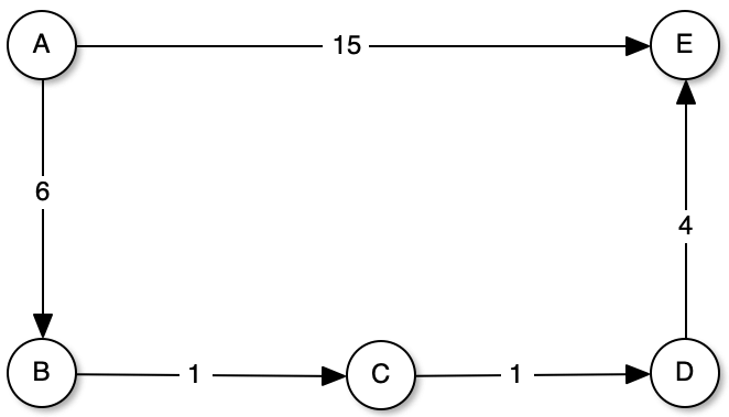
Let's try the shortest path from A to E. As we can see, the straight path has a weight of 15, however, if we go through the nodes A-B (6), B-C(1), C-D(1) and D-E(4) that adds up to a total weight of 12, which means that this path, despite having more nodes, has a lower cost.

Example - shortest path using the dijkstra algorithm

The below classes are extracted from the Dijkstra library on GitHub.

# If we install the dijkstra library, we can import the classes as usual.
# from Dijkstra import DijkstraSPF, Graph

Let's create a simple graph to test the Dijkstra shortest path algorithm.

Let's try the shortest path from A to E. As we can see, the direct path has a weight of 15, however, if we go through the nodes A-B (6), B-C(1), C-D(1) and D-E(4) that adds up to a total weight of 12, which means that this path, despite having more nodes, has a lower cost.

label distance
A     0.000000
B     6.000000
C     7.000000
D     8.000000
E     12.000000

Shortest path:
A -> B -> C -> D -> E

If we change the weight of segment [A, E] from 15 to 10, the algorithm has a direct path to the node E.

Shortest path:
A -> E

As we can see, Dijkstra's greedy algorithm is an optimal solution for finding shortest paths in a directed graph. However, it is not a valid algorithm for arbitrage since, having to normalise the prices to a logarithmic scale, we can obtain negative values for the weights. With the Dijkstra algorithm we would obtain infinite cycles, for which the Bellman-Ford algorithm is used.

Why does the Dijkstra algorithm fail for negative weights?

Dijkstra's algorithm fails for graphs with negative edge weights because it assumes that once a shortest path to a node has been found, it cannot be improved. This assumption breaks down when negative weights are present, as a shorter path might be found later that reduces the overall distance. Specifically, negative weights can lead to scenarios where the algorithm incorrectly finalises the shortest path to a node, missing out on potentially shorter paths that include negative edges.

Negative weights can also lead to negative weight cycles, where the total weight of a cycle (loop) is negative. In such cases, one could traverse the cycle indefinitely to decrease the path cost infinitely, which Dijkstra’s algorithm is not designed to handle. This issue is critical in certain applications, requiring specialised algorithms such as the Bellman-Ford algorithm or Johnson’s algorithm to correctly handle negative weights and detect negative weight cycles.

One of the applications we have of the Dijkstra algorithm is currency arbitrage. The Real Effective Exchange Rate (REER) is an index used to assess the value of a currency relative to a basket of other currencies, adjusted for inflation. While the REER itself does not directly relate to the mechanics of shortest path algorithms, understanding exchange rates and their impacts on trading decisions can be crucial for constructing accurate models in quantitative finance.

References

Fundamentals of algorithmics by G. Brassard and P. Bratley
Princeton University, Dijkstra's algorithm and Bellman-Ford algorithm
scipy.sparse.csgraph.dijkstra library
Arbitrage Strategy using Negative Cycle Detection Algorithm
Currency aribitrage detection

Conclusion

As we have seen, the Dijkstra algorithm finds the optimal solution to obtain the shortest path in a graph from an origin to the rest of its nodes. This algorithm has applications in countless problems that can be represented as a graph or tree.

It differs from the Kruskal algorithm and Prim algorithm in that they focus on discovering the minimum coverage tree, i.e., how to cover the entire graph efficiently, while the Dijkstra algorithm focuses on optimising the shortest path where it is not necessary to cover all the edges of the graph but to reach all the nodes. Finally, we have seen that the Dijkstra algorithm has problems such as negative weights for the edges, for which the Bellman-Ford or Johnson algorithms are used.

Dig into the world of algorithms and trading, and start your quest to upgrade your knowledge of Algorithmic Trading with our comprehensive algo trading course, the Executive Programme in Algorithmic Trading (EPAT) which covers topics ranging from Statistics & Econometrics to Financial Computing & Technology including Machine Learning and more. Be sure to check it out!

Author: Mario Pisa

Disclaimer: All investments and trading in the stock market involve risk. Any decisions to place trades in the financial markets, including trading in stock or options or other financial instruments is a personal decision that should only be made after thorough research, including a personal risk and financial assessment and the engagement of professional assistance to the extent you believe necessary. The trading strategies or related information mentioned in this article is for informational purposes only.

AOV Course Launch