Exploratory data analysis (EDA) is when you use the available data and try to visualise it in different forms and use various permutations and combinations to become familiar with the data and derive meaningful observations. After completing your EDA, the logical next step is technical analysis in Python applying computed indicators like moving averages, Bollinger Bands, and RSI to the cleaned dataset to generate trading signals. It is the step after we have cleaned and prepared the data but before we start the data modelling. But why can’t we move directly to the data modelling part?
Well, when you think about it, you actually can skip the Exploratory data Analysis part. But if you weren’t familiar with the data, you wouldn’t know which variable could have the highest impact and thus make it easy to solve the problem statement. It’s as simple as that.
“Far better an approximate answer to the right question, which is often vague, than an exact answer to the wrong question, which can always be made precise.” - John Tukey
Yes, exploratory data analysis does help us in getting the answer faster. Let’s move further and see the topics we are going to cover in this blog.
What is Exploratory Data Analysis?
It is said that John Tukey was the one who introduced and made Exploratory data analysis a crucial step in the data science process. When asked what does it mean, he simply said, “Exploratory data analysis" is an attitude, a state of flexibility, a willingness to look for those things that we believe are not there, as well as those we believe to be there.”
The main aim of exploratory data analysis is to:
- Gain insight into the available data
- Find out any relation between the different variables
- Find anything which is out of the ordinary, ie outlier or anomaly
- Test any assumptions or instincts
- Find any optimum parameters or variable which will help us solve the problem statement faster
Yes, that’s probably it. You can see where the EDA process stands in the whole data science process below

The main component in exploratory data analysis is the visualisation of data. Let’s see how we perform Exploratory Data Analysis in the next section.
What are the types of EDA methods?
Existing literature tells us that there are four types of exploratory data analysis. Let’s look at them below:
Univariate non-graphical method
Breaking down the name, univariate implies that there is just one variable and non-graphical is well, there is no visual element in this method.
There are plenty of examples in this method, which can vary from the height of NBA players in a team or only the opening price of Tesla Inc. in 2019. One of the Univariate non-graphical methods can be the 5 number summary of a variable.
Taking the example of Tesla Closing prices for 11 days, we will take only the closing prices and tabulate them below. Thus it would look something like this:
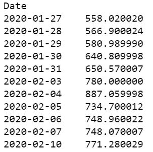
The five-number summary consists of the Minimum value, 1st Quartile, Median, 3rd Quartile, and Maximum number.
Let’s calculate this in Python:
You will get the following output:

Of course, apart from the following, you can always check the number of values, the mean etc.
By the way, you can also try the one-line command which pretty much gives you all the information you need in a simple format.
The python code is:
tesla['Close'].describe()

You can also find the standard deviation and the variance with the “statistics” package. The python code is shown below:
The output is as follows:

Univariate graphical method
Let me ask you a question, have you ever asked a friend for directions to their house and felt confused. Sure they are giving the right directions, “Take a left turn at XYZ Mall and a right at the ABC Bank” etc., but you can’t help feeling that it could be better. What if the friend gives you a map and says they have circled the destination in red.”
Well, the map sounds better right? Most of us are quick to learn something if we have a visual in front of us than plain numbers in a table.
Hence, we will take the earlier example, and do a line plot of the closing price to see the trend in the market.
The python code is as follows:

You can also use the histogram to see the distribution. We will find the daily returns and plot its histogram.
Let’s see the histogram:
tesla['daily_returns'].dropna()
plt.hist(tesla['daily_returns'], bins = 5)
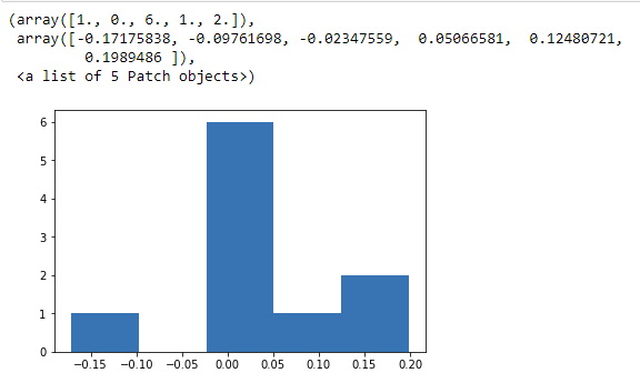
Since it is a small data set, we can’t really infer anything meaningful here. In contrast, if we do a histogram of Tesla for the last year, we will find it as follows:

Ok, so we used the ‘dropna’ method because it interferes with our calculations when we are analysing the data. Sometimes, people feel we shouldn’t drop the whole row as it might contain some other information as well. And part of exploratory data analysis is to handle the missing values too.
While we don’t have to do this for our example, we can use the ‘fillna’ method to handle the missing values. But what values do we put in so that it doesn’t mess with our analysis?
A simple workaround is to fill the values with the mean of the dataset so that the final analysis is not modified.
Hypothetically if we had a missing value in the “Close” column, and we know the mean is 697.03, we will put the following code:
tesla['Close']=tesla['Close'].fillna(697.03)
Yes. And just with this simple line of code, we can fill any columns which are “NaN” etc.
Remember how we did the five-number summary of Tesla for 11 days. Well, we can represent it in the form of a boxplot as well. The code is as follows:
tesla.boxplot(column = 'Close');
plt.title('')

All right! Let’s move on to the next one.
Multivariate nongraphical method
So far we were working on just one variable. But in reality, we have more than one variable to contend with. Thus, we move to the next method, ie multivariate non-graphical methods. If we had to pick the best NBA team from the available players, we wouldn’t just look at their heights, right?
We take into account multiple variables such as their experience, matches played, matches won, successful baskets, scores, medical history etc. This would give us a better shot at picking the ultimate team to win the NBA. In a similar manner, we have the Tesla stock price which consists of the following parameters: Date, Opening price, Closing price, High, Low and Adj Close, Volume and the daily returns we had calculated.
Now, just like the univariate analysis, we can use the “describe” function here too, giving us a chance to have a quick glance on the data.
The python code will be as follows:
tesla.describe()

This helps us know how different the variables are in comparison to each other. There is one more function which helps us get an overview of the data we have. The Python code is quite simply,
tesla.info()

You can see which variables have any null values or not. As you know, having null values can sometimes become an obstacle for effective analysis. All right, let’s move on to the heart of the matter.
Multivariate graphical method
In multivariate graphical methods, we will analyse the entire dataset together. The main component of the multivariate graphical method is probably the scatterplot. Scatter plots are used to visualize the relationship between two different data sets. There is a great line of code which plots scatter plots of all the variables with respect to each other as well as others. The code is as follows:
pd.plotting.scatter_matrix(tesla, alpha=1.0, figsize=(20, 20), diagonal='kde')
plt.show()

The scatter plot is an interesting way to look at the entire dataset and observe any correlations, or lack thereof. In addition to scatterplots, we also have heatmaps which are a two-dimensional graphical representation of data where the individual values that are contained in a matrix are represented as colours. The “seaborn” python package allows the creation of annotated heatmaps which can be tweaked using Matplotlib tools as per the creator’s requirement.
You can learn how to create a heatmap using seaborn in this step-by-step tutorial.
For our example, we will use the seaborn package as well and create a heatmap with the following code:
import seaborn as sns
plt.figure(figsize=(10,10))
sns.heatmap(tesla.corr(),cmap='Oranges',annot=False)
The output is as follows:

I think we have covered a lot of the methods which are used in exploratory data analysis. Of course, there are literally dozens of charts and graphs which can be created using Python, the Python Graph Gallery being a good resource. Did we miss anything? Let us know in the comments below and we would be more than glad to add them to this blog.
Conclusion
Exploratory Data Analysis is an important part of the data scientist as it helps to build a familiarity with the data we have available. Using EDA will help us in arriving at the solution much faster as we would have already identified any patterns which we would like to exploit when we enter the data modelling phase. Spending some time with the data will also help us gain any insights which we would have probably missed if we had gone directly to the data modelling part.
We have created a beginner level course for individuals who want to start out on their journey in data science. Do check it out now for free.
Download Data File
- Exploratory Data Analysis in Python.ipynb
Disclaimer: All investments and trading in the stock market involve risk. Any decisions to place trades in the financial markets, including trading in stock or options or other financial instruments is a personal decision that should only be made after thorough research, including a personal risk and financial assessment and the engagement of professional assistance to the extent you believe necessary. The trading strategies or related information mentioned in this article is for informational purposes only.