Implied Volatility: Formula, Options, Python, Calculations and more

Have you ever wondered how to gauge the market's anticipation of volatility? Is there a method to predict future volatility, aiding us in strategic moves within the options trading domain? Let us find out the answers to all these questions in this blog ahead that covers implied volatility in detail.

"When a long-term trend loses its momentum, short-term volatility tends to rise."
- George Soros

Intriguing, isn't it?

In the ever-fluctuating financial markets, volatility plays a pivotal role in influencing the pricing and behaviour of financial instruments. Among the various facets of volatility, one key metric takes centre stage: Implied Volatility (IV). Implied volatility serves as a crucial indicator, reflecting the market's expectations regarding future price fluctuations. Understanding and effectively utilising implied volatility is essential for informed decision-making, especially in options trading where it directly impacts option prices and strategies. You can explore the course on options trading course by Quantra.

Volatility, in essence, captures the price movements - both upward and downward - of financial assets. It reflects the market's uncertainty, influenced by factors such as supply and demand dynamics, sentiment, and external events like economic shifts or crises. Implied Volatility, a forward-looking measure, gauges the market's anticipation of future price swings, specifically in the options market.

This journey into Implied Volatility involves delving into its interpretation, distinguishing it from historical and realised volatility, exploring the mathematical intricacies behind its calculation, and understanding the impact of various market factors. Implied Volatility isn't just a singular concept; it's a versatile tool employed by traders for diverse purposes, from option pricing and market expectation assessment to implementing sophisticated trading strategies.

This blog covers all major topics of implied volatility in options trading but, before we dive into the basics of implied volatility, you should be aware of the options trading basics.

This blog covers:

Understanding implied volatility
How to interpret implied volatility in options trading?
Implied volatility vs historical volatility
Implied volatility vs realized volatility
How to calculate implied volatility?
Calculating implied volatility using Python
Uses of implied volatility
Challenges and risks of using implied volatility in trading
Tips for the traders to overcome challenges

Understanding implied volatility

We will first start with a brief introduction of volatility in order to learn the implied volatility from the start.

Volatility

Volatility is one of the most important pillars in financial markets. In simple words, volatility refers to the upward and downward price movements (fluctuations) of a financial asset. The movements are due to several factors including demand and supply, sentiment, corporate actions, greed, and fear, etc. Some common examples of volatility in trading are the COVID-19 pandemic, the 2008 financial crisis etc.

Now that we know what volatility is, let us now understand what implied volatility means!!

Implied volatility meaning

Implied volatility (IV) is the measure of expected future volatility in the options market. Essentially, implied volatility was and is still considered to be an integral component of the Black-Scholes-Merton model (a popular option pricing model), where it represents future volatility associated with the underlying asset.

But, did you know that it is not the only type of volatility measure available in the market?

One most common type to measure volatility is realized volatility, also known as historical volatility (HV). (Learn advanced volatility trading in detail in the Quantra course).

Realized Volatility or historical volatility (HV)

Historical volatility indicates the deviation or change in prices of the underlying asset over a given period in the past. Usually, historical volatility is calculated over one-year i.e. 252 trading days. It is used by traders to compare the current volatility level of an underlying asset with its historical volatility.

Whenever there is a gap between the current and historical volatility, traders take positions based on the opportunity. However, the issue with historical volatility is that it is a backwards-looking indicator which means it is based on past returns and is not the most reliable form of volatility.

You can also take a look at this interesting introductory video on implied volatility beginning with the insights on volatility so as to cover the basics:

How to interpret implied volatility in options trading?

The value of implied volatility has been factored in after considering market expectations. Market expectations may be major market events, court rulings, top management shuffle, etc.

If you want an in depth know how into volatility options trading, you can refer to this webinar below by Dr. Euan Sinclair.

In essence, implied volatility is a better way of estimating future volatility in comparison to historical volatility, which is based only on past returns. Also, there is more than one way to visualise and interpret implied volatility and we will look at each one of them specifically.

So, let us begin!

Data Table

The most basic way to visualise implied volatility numbers would be through a data table format. Now, in the options market, it is known as an option chain.

Example: AAPL Implied Volatility Skew with data table

Below is an Option Chain for the US Stock: Apple (ticker: AAPL)

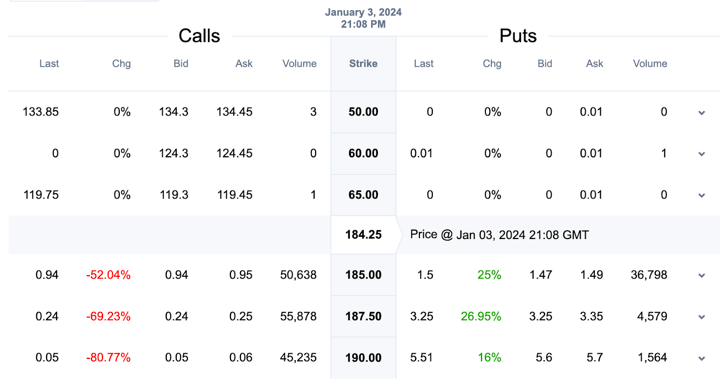
From the above image, it is very clear that the Implied Volatility for the same strike price is different for call and put options. Also, for different strike prices, the Implied Volatility fluctuates with the shift in market expectations.

Note: Implied Volatility is not a direction-based parameter and therefore it only indicates the range of prices an underlying asset might move in the future.

This change in implied volatility in both the put and call option at different strike prices is characterised by "Volatility Smile" and “Volatility Skew”.

Volatility Smile takes place when the implied volatility is the highest at OTM and ITM call or put options with the lowest at, ATM option.
In the case of Volatility Skew, is where different strike prices have different implied volatility for the same underlying asset.

Both interpretations are used in the options market for better visualisation purposes. Below, we have mentioned the Volatility Skew example from the call option strike prices and implied volatility relatively.

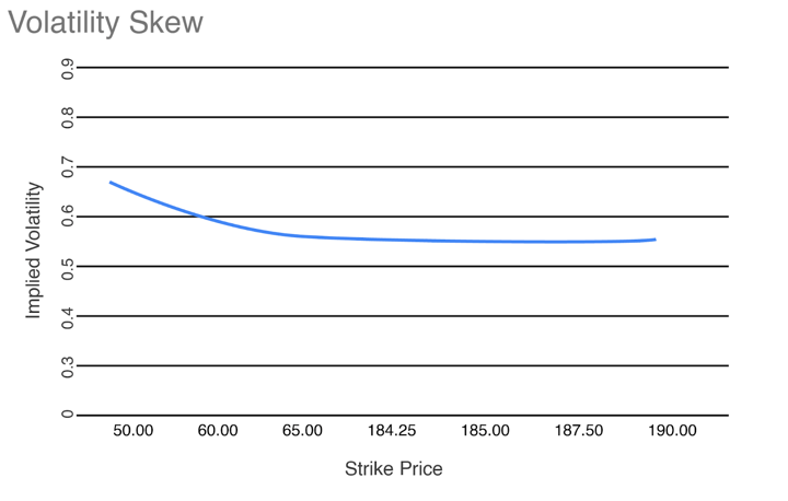
Alright, now that we have understood and interpreted implied volatility from an options chain data table, we will visualise implied volatility through a chart and interpret implied volatility levels from the same.

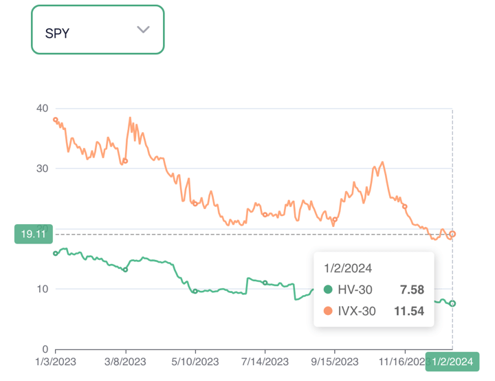
Volatility chart — Source: IVolatility.com

In the chart, we have the implied (IVX) as well as 30-day historical volatility (HV) data for the past one year.

Market participants use historical implied volatility levels to gauge an understanding of where the implied volatility, say, for example, was at 3 months ago and at what level it is today for trading based on the opportunity.

Traders also use past trends of both historical and implied volatility to understand if the historical volatility and implied volatility together are higher or lower than in previous periods. If you start trading options today, this is your go-to tool for gauging implied volatility levels. As stated earlier, there are many factors why the implied volatility level is high or low at a certain point in time.

Implied Volatility Rank (IVR)

Implied Volatility Rank is a popular way of calculating the implied volatility over the last one year or 52 weeks. It is calculated to figure out how high or low the current implied volatility level is when compared with the annualised levels.

Formula to calculate the Implied Volatility Rank:

The formula to calculate IV Rank is:

Current implied volatility% - 52 weeks low implied volatility %/ 52 week high implied volatility% - 52 weeks low implied volatility%

Calculating AAPL Implied Volatility Rank:

Let’s consider the example of Apple (ticker: AAPL) which was mentioned in the chart section of implied volatility. The current implied volatility is at 32.5%, 52 week low implied volatility is 18%. 52 week high IV is 34%.

So let’s do the maths:

32.5% - 18% / 34% - 18% = 14.5% / 16% = 90.625%.

Interpreting the Implied Volatility Rank is easy too. Intuitively Implied Volatility Rank refers to the difference between the current implied volatility and 52 week low implied volatility. In this case, it is 90.625%. This means that the implied volatility is currently high enough and a trader would be interested in selling the options due to the high implied volatility.

High implied volatility means high option price and thus would benefit the option sellers heavily. Option buyers who buy options with high implied volatility face losses due to the decrease in implied volatility at a later point in time.

Implied Volatility Percentile (IVP)

Implied Volatility Percentile is another interesting way to look at implied volatility or to interpret it. Implied Volatility Percentile simply refers to the number of days the current implied volatility is under the current implied volatility percentage value as compared to the total number of trading days ie. 252 trading days.

Formula to calculate the Implied Volatility Percentile:

Implied Volatility Percentile = Number of trading days under current implied volatility / Number of trading days in a year.

Calculating AAPL Implied Volatility Percentile:

For example, if the number of days under the current implied volatility (30%) is 100. The number of trading days is 252.

Implied Volatility Percentile = 100/252 = 39.68 percentile (approx).

Below is a data table of stocks dated for the 13th of December, 2023 with their Implied Volatility Rank and Implied Volatility Percentile for visualising IVR and IVP!

Symbol	Implied Volatility Rank	Implied Volatility Percentile	Implied Volatility
Tesla Inc (TSLA)	15.18	5	43.88
Adv Micro Devices (AMD)	12.90	4	37.12
Nvidia Corp (NVDA)	3.22	2	33.21
Apple Inc (AAPL)	0.00	0	15.76
Amazon.com Inc (AMZN)	1.04	0	23.61

Example: AAPL implied volatility vs AMZN implied volatility

Let us deduce the concept of IVP with relation to Implied Volatility with an example of two equity stocks i.e. Apple Inc (AAPL) and Amazon.com Inc (AMZN).

AAPL has an Implied Volatility (IV) of 15.76 % whereas AMZN has an Implied Volatility of 23.61%. Given that there is a huge gap between the implied volatility of both the equity stock options, to the logical mind, it looks like the IVP should have a huge difference too.

However, in reality, the IVP of both AAPL and AMZN is “0”, which is the same!

Therefore, before trading options using implied volatility, one should be aware of the historical implied volatility values for an option and where it stands currently.

This is exactly where the application of the Implied Volatility Percentile becomes crucial, where it helps us in identifying current implied volatility values in comparison to where the implied volatility has been over the past one year (252 trading days).

You can also take a look at this video below that covers implied volatility from theory to practice:

Implied volatility vs historical volatility

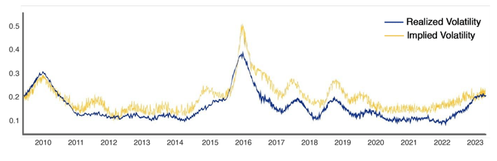
In the below example, we show the Dow Jones Index’s comparison between Implied Volatility and realized volatility (volatility that actually took place) to visualise the same concept.

The blue line represents realized volatility and the yellow line represents implied volatility.

Implied Volatility is mostly above the realized or historical volatility due to fluctuation in market expectations.

Now, let us briefly see the difference between implied volatility and historical volatility.

Aspect	Implied Volatility (IV)	Historical Volatility (HV)
Definition	Represents expected future price volatility from options	Measures past price fluctuations using historical data
Calculation	Obtained from option pricing models (e.g., Black-Scholes)	Calculated from historical price movements
Use in Options Pricing	Crucial; higher IV leads to costlier options	Not directly used in options pricing
Market Expectations	Reflects current market sentiment and expectations	Provides insights into historical movements
Dynamic Nature	Dynamic, changing rapidly based on market conditions	Static, representing past volatility over a period
Trading Strategy	Used to identify potential mispricing and trading signals	Helps assess whether current implied levels deviate from historical averages

Example of Implied volatility vs Historical volatility:

Scenario	Implied Volatility	Historical Volatility
An earnings report is approaching, causing uncertainty.	Rises as traders expect increased volatility; options prices increase.	May not capture the anticipation, as it reflects past data.
Market News Impact	Reacts quickly to breaking news, adjusting to the market's changing expectations.	Reflects historical news impact, not immediate reactions.
Stable Market Periods	Tends to be lower during stable market conditions.	Captures past stability but may not provide insight into current sentiment.

Implied volatility vs realized volatility

Realized volatility refers to the measure of daily changes in the price of a security over a particular period. Realized volatility’s calculation requires the continuously compounded daily returns to be calculated first of all.

It assumes the daily mean price to be zero to provide movement regardless of direction. It is different from Implied volatility in the sense that realized volatility is the actual change in historical prices, while implied volatility predicts future price volatility.

Aspect	Implied Volatility (IV)	Realized Volatility (RV)
Definition	Expected future price volatility from option prices	Actual historical price volatility based on realized data
Calculation	Obtained from option pricing models (e.g., Black-Scholes)	Calculated from historical price movements
Use in Options Pricing	Critical; affects option prices, higher implied volatility means costlier options	Not used directly in options pricing
Market Expectations	Reflects current market sentiment and expectations	Indicates how much the asset has moved historically
Dynamic Nature	Dynamic, influenced by real-time market events	Static, reflecting historical movements over a period
Accuracy in Predictions	Reflects traders' expectations about future volatility	Provides an accurate measure of actual past volatility
Trading Strategy	Used for identifying potential mispricing and trading signals	Not used directly for trading decisions, but informs about past volatility

Example of Implied volatility vs Realized volatility:

Scenario	Implied Volatility	Realized Volatility
Earnings Announcement	Rises before an earnings report as traders anticipate increased volatility.	Measures the actual volatility post-earnings, capturing the realized impact.
Market Calm Periods	May remain low during calm market conditions.	Reflects historical stability, showing how much the market actually moved.
News-Driven Events	Reacts quickly to breaking news or events, adjusting based on market expectations.	Shows the real impact of the news on price movements after it occurs.

Understanding the distinction between implied and realized volatility is essential for traders to make informed decisions, balancing market expectations and compounded historical data (daily returns).

How to calculate implied volatility?

We will now move forward and understand the mathematics behind implied volatility and how it is calculated for options.

Calculating implied volatility is not as easy a task as it might appear to be. To calculate the implied volatility of a call or put option, we first need to understand the mathematics behind the Black Scholes Merton(BSM) Model.

As for this article, we will not dig down much into the concept of the BSM Model but we will have an overview of what is the BSM model so that the calculation of implied volatility looks similar and easy to understand.

Black Scholes Merton Model

The Black-Scholes-Merton model is the most popular option pricing model used by traders when it comes to European options. It has two separate formulas for calculating the call option and the put option.

The Parameters for calculating the call option are:

St – Spot Price of the underlying asset (Current Price)
K – Strike Price of the underlying asset
r – Risk-free rate(continuously compounded)
σ – Volatility of returns of the underlying asset
T-t – Time to maturity (in years)
N – Cumulative distribution function of Normal Distribution

Pricing the call option:

$$C(S_t,t) = N(d_1)S_t - N(d_2) PV(K)$$$$d_1 = \frac{1}{σ\sqrt (T-t)}$$$$d_2 = d_1 - σ \sqrt (T-t)$$ $$PV(K) = {K_e^-r}^{(T-t)}$$

Pricing the put option:

$$P(S_t,t) = {K_e^-r}^{(T-t)} - S_t + C(S_t,t)$$ $$=N(-d_2){K_e^-r}^{(T-t)} - N(-d_1)S_t$$

Looks a bit complicated right? Don’t worry, once you input the values of the parameters it will be easier to calculate.

For example: If the parameters are as follows.

Spot Price (St): 300 Strike Price (K): 250 Risk-free rate (r) = 5% Time to maturity (T-t) = 0.5 years (6 months) Call Price = 57.38

How do we find the implied volatility for the call option with the parameters as mentioned above?

We will simply use the method of reiteration or trial and error. This iteration is needed because the Black-Scholes formula is not directly solvable for implied volatility algebraically. It involves the cumulative distribution function of the standard normal distribution, and finding the inverse of this function is not straightforward.

The iterative process involves making an initial guess for implied volatility, calculating the option price using the Black-Scholes formula, and then adjusting the implied volatility until the calculated price converges to the observed market price.

This iterative approach is often more practical than attempting to solve for implied volatility algebraically.

In summary, while it is theoretically possible to substitute the call price into the Black-Scholes formula and solve for implied volatility, the iterative approach is commonly used in practice because it's more efficient and numerically stable.

If we guess the implied volatility is 15%, we get a call option price of 56.45.

If we guess it's 25%, the price is 59.

By trying different guesses, we see that an implied volatility of 20% gives a price of 57.38.

So, based on these tests, the implied volatility seems to be between 15% and 25%, possibly around 20%. The same technique can be used to put options accordingly. Once you get hold of this technique, it's as easy as pie!

Calculating Implied Volatility using Python

Alright, now that we know the concept of implied volatility, why not create a calculator for calculating implied volatility of an option?

After all, the knowledge earned should be applied practically!!

We will create an implied volatility calculator using Python for easy calculation of implied volatility for an option.

The Python Code:

Output for the input code:

18.24951171875

This means that the implied volatility for the call option is 18.249% (approx).

Wasn’t that simple?!

Python calculates a complex mathematical model such as the Black-Scholes-Merton formula very quickly and easily. This same mechanism can be used to calculate put option implied volatility.

Factors affecting implied volatility in the market

Let’s take a look at certain factors that influence implied volatility in options trading:

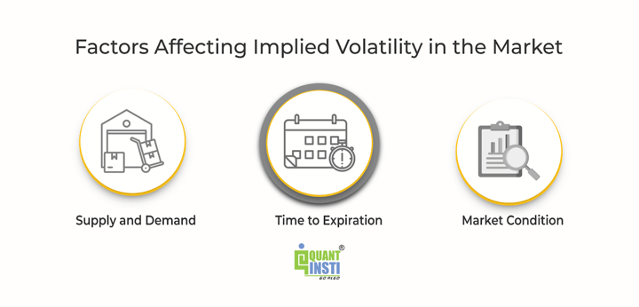
Supply and Demand

With the increase in the demand for an underlying asset, the implied volatility increases too and so does the option price! Of course, this phenomenon is exactly the opposite when the demand is low. High IVs tend to move towards the mean implied volatility value with the fall in demand and the supply starts stabilizing concurrently. This all takes place once the market expectation starts falling and leads to a reduction in the option price.

Time to Expiration

Time to expiration, better known as theta, which measures the amount of time left for the option to expire, affects the implied volatility of an option directly.

Implied volatility and short time to expiry - Generally, as the time to expiry decreases, implied volatility tends to increase. This is because as an option approaches expiration, uncertainty about its future movements may rise, leading to higher implied volatility.
Implied volatility and longer time to expiry - Conversely, when the time to expiration is relatively longer, implied volatility might be lower. This is because there is more time for the underlying asset to make significant price movements, and the uncertainty or risk of those movements is spread out over a longer period. Therefore, options with longer expiration times may have lower implied volatility.

Market condition

Most underlying assets are directly impacted by the market sentiment or events that are to take place in the future for a listed organisation. Earnings announcements, court rulings, top management shuffles, etc are some of the market events that lead to high IV with an option as the market is unsure of the direction that the underlying asset might move.

Uses of implied volatility

Implied volatility is certainly used frequently in the options market by traders. The listed below are the various uses of implied volatility:

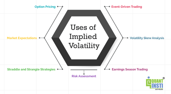
Option Pricing - Implied volatility influences the pricing of options. Higher implied volatility suggests a higher likelihood of significant price swings, leading to more expensive options. Traders consider this when evaluating the cost and potential profitability of options contracts.
Market Expectations - Implied volatility reflects the market's anticipation of future price movements. Rising implied volatility may indicate expectations of upcoming events, such as earnings reports or economic releases, influencing trading decisions.
Straddle and Strangle Strategies - Traders employing straddle or strangle strategies seek to benefit from significant price movements. Implied volatility is a key factor in choosing appropriate conditions for these strategies, as higher volatility increases the potential for larger price swings.
Risk Assessment - Implied volatility is a crucial factor in assessing the risk associated with a stock or option. Traders analyse implied volatility to gauge the potential for price fluctuations and adjust their risk management strategies accordingly. Hence, the role of implied volatility in risk management is quite crucial.
Earnings Season Trading - Implied volatility often rises during earnings season due to uncertainty. Traders monitor implied volatility to anticipate potential price movements and adjust their positions or employ strategies that capitalise on increased volatility.
Volatility Skew Analysis - Implied volatility can vary among different options contracts for the same asset. Traders analyse volatility skew to identify potential mispricings, helping them choose options with favourable risk/reward profiles.
Event-Driven Trading - Before significant events, implied volatility tends to increase. Traders utilise this information to anticipate potential price changes driven by events such as mergers, acquisitions, or regulatory decisions.

Challenges and risks of using implied volatility in trading

Below are some challenges and risks of using implied volatility in trading.

Challenges and Risks of Using Implied Volatility in Trading	Explanation
Market Noise	Fluctuations in implied volatility may be driven by market noise rather than genuine changes in the expected volatility.
Model Assumptions	Implied volatility calculations rely on option pricing models with certain assumptions, and deviations can impact accuracy.
Limited Historical Data	Limited historical data for some securities can affect the accuracy of implied volatility calculations.
Event Risk	Unexpected events, such as geopolitical developments, can lead to sudden and significant changes in implied volatility.
Over Reliance on implied volatility	Relying solely on implied volatility without considering other factors may lead to suboptimal trading decisions.
Dynamic Nature of implied volatility	Implied volatility is dynamic and subject to rapid changes, requiring traders to adapt quickly to shifting market conditions.
Volatility Smile/Smirk	Different options on the same underlying asset may exhibit varying implied volatility patterns, challenging uniform analysis.
Market Sentiment Mismatch	Traders must interpret whether high implied volatility reflects fear or opportunity, as it can indicate both.

Tips for the traders to overcome challenges

Below are some useful tips for the traders to overcome the challenges that surround using implied volatility in trading.

Tips	Explanation
Diversify Strategies	Employ a mix of strategies that consider implied volatility but also account for other factors, reducing reliance on a single approach.
Continuous Learning	Stay informed about market dynamics, events, and economic indicators to better interpret and adapt to changing implied volatility.
Use Multiple Indicators	Combine implied volatility analysis with other technical and fundamental indicators for a comprehensive view of market conditions.
Risk Management	Implement robust risk management strategies to mitigate the impact of unexpected events and sudden changes in implied volatility.
Monitor Market Sentiment	Regularly assess market sentiment through news, social media, and other sources to understand the context of changing implied volatility.
Test and Validate Models	Regularly test and validate option pricing models against historical data to ensure accuracy and reliability in various conditions.
Stay Disciplined	Stick to predefined trading plans and avoid impulsive decisions based solely on implied volatility changes, maintaining discipline in strategy execution.
Understand implied volatility Patterns	Learn to interpret different implied volatility patterns, such as the volatility smile or smirk, to make more informed trading decisions.
Adapt to Market Conditions	Recognize that market conditions can evolve, requiring flexibility in trading strategies and the ability to adapt to changing implied volatility dynamics.
Leverage Technology	Utilise advanced trading platforms and analytics tools that provide real-time implied volatility data, helping traders make more informed and timely decisions.

Conclusion

Implied volatility is a crucial aspect of options trading, representing expected future price volatility. Traders use it for option pricing, risk assessment, and various strategies. Understanding IV involves comparing it with historical and realized volatility, visualising it through data tables and charts, and calculating it using the Black-Scholes-Merton model.

Market factors like supply and demand, time to expiration, and market conditions influence IV. Despite its utility, traders face challenges such as market noise and model assumptions. To navigate these challenges, diversifying strategies, continuous learning, and leveraging technology are essential, ensuring a disciplined and adaptive approach in dynamic markets.
For those new to trading, exploring volatility trading strategies for beginners is an excellent starting point to build confidence and expertise in navigating market complexities.

If you wish to explore options volatility in more depth, you could explore our course on Options Volatility in Trading. This course has topics like options Greeks, volatility estimators (Garman-Klass and Parkinson), GARCH modelling. Moreover, you can learn to do the analysis of PnL distribution for popular strategies like straddles and strangles.

With a hands-on capstone project and a live trading template in this course, you'll gain practical experience applying these concepts in real-life scenarios. So, join us on this options volatility trading journey today!

Author: Chainika Thakar (Originally written By Punit Nandi)

Note: The original post has been revamped on 15th January 2024 for accuracy, and recentness.

Disclaimer: All data and information provided in this article are for informational purposes only. QuantInsti^® makes no representations as to accuracy, completeness, currentness, suitability, or validity of any information in this article and will not be liable for any errors, omissions, or delays in this information or any losses, injuries, or damages arising from its display or use. All information is provided on an as-is basis.

Free Algo Trading Beginner Courses