Applying LightGBM to the Nifty index in Python

By Manusha Rao

LightGBM is gaining popularity recently since it is faster than other gradient boosting algorithms. In this article we will see how LightGBM algorithm is used to predict the NIFTY50 daily moves.

• What is LightGBM?
• Working principles of LightGBM
• Why is LightGBM gaining popularity?
• LightGBM parameters overview
• Implementation of LightGBM in Python

What is LightGBM?

LightGBM stands for Light Gradient Boosting Machine. LightGBM is based on gradient boosting that uses a tree-based machine learning technique. It is considered to be fast compared to other similar algorithms.

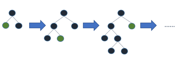
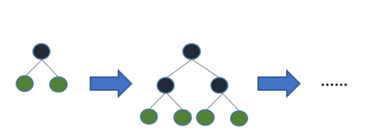
You might wonder, there are already so many tree-based algorithms, so what is the big deal about LightGBM? The difference in this algorithm is that the tree grows vertically (i.e. leaf wise), whereas the other tree based algorithms grow horizontally (i.e. level-wise) as demonstrated in the images below.

Working principles of LightGBM

LightGBM is based on two main principles which set it apart from all gradient boosting algorithms:

Gradient One-Sided Sampling(GOSS)

In this technique, more attention is given to samples with higher gradients(i.e., more loss). Let's dive a bit deeper into this concept.

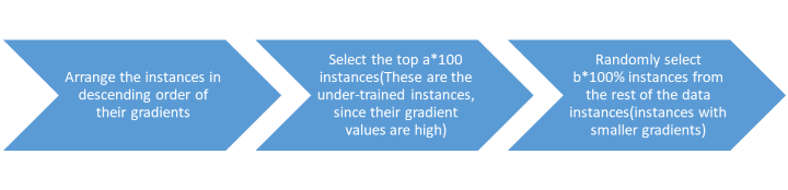
Consider a base model which is used to train 500 samples. After training, we will have 500 errors {X1, X2, X3,......X500}. Now GOSS sorts these errors in descending order, i.e. the highest absolute error value to the lowest.

Then, the top a% instances with the larger gradients are kept, and the instances with lower gradients in the remaining (1-a)% instances i.e., b% are randomly chosen. This ensures that the weak learners are given more importance.

Exclusive Feature Bundling(EFB)

Machine learning models typically have many features. What if we can reduce the number of features so that the speed improves?  LightGBM offers exactly that. Let’s break down the EFB into two parts:

1). Bundling similar features together - Using a weighted graph, the features are bundled together

2). Merging the features together - After bundling, we will merge features that cannot take zero values simultaneously.

Let us understand this with the help of a simple example.

Consider a machine learning model that is trying to assess the investor risk-aversion based on a number of features(inputs). Consider two features ‘male’ and ‘female’. Since these features can never take zero values simultaneously we can merge them into one feature. As a result, two features have been reduced to one.

Why is LightGBM gaining popularity?

Some of the reasons why LightGBM algorithm is attracting a lot of attention are:

Handles large datasets

LightGBM is known for handling large datasets better than XGBoost.

Faster training speed

As it is pretty evident from the below code snippets, LGBM is 4 times faster than XGBoost.

Output:

CPU times: total: 578 ms
Wall time: 138 ms

LGBMClassifier(learning_rate=0.01, max_depth=5, n_estimators=200, num_leaves=80)

Output:

CPU times: total: 2.44 s
Wall time: 461 ms

XGBClassifier(base_score=0.5, booster='gbtree', callbacks=None, colsample_bylevel=1, colsample_bynode=1, colsample_bytree=1, early_stopping_rounds=None, enable_categorical=False, eval_metric=None, feature_types=None, gamma=0, gpu_id=-1, grow_policy='depthwise', importance_type=None, learning_rate=0.01, max_depth=5, n_estimators=200, num_leaves=80)

Less memory usage

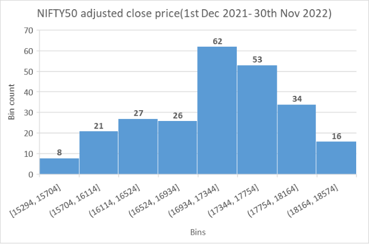
LightGBM achieves this through a technique known as binning. Now, what is binning? Binning is a process where a continuous variable/feature (such as stock prices) is converted into a discrete set of bins. Consider NIFTY50 adjusted close price data from 1st December 2021 to 30th November 2022 (that is approximately 252 trading days).

We have 252 data points(adjusted close prices), which would require a considerable amount of memory. In order to reduce the memory used, I have demonstrated the binning technique with the help of Excel. Here, the prices are sorted into 8 different bins(X-axis). The Y-axis represents how many values lie in each bin.

The count is displayed on the top of each bin. This way, 252 data points are categorized into eight bins, resulting in reduced memory utilization.

Supports GPU learning

GPUs support parallel processing. This type of processing entails breaking down significant complex problems into smaller tasks that can be processed simultaneously.

Easier to encode categorical features

When we talk about categorical value representation, the first thing that comes to mind is one-hot encoding. However, LightGBM uses a more efficient and faster algorithm to automatically deal with categorical values provided they are integer encoded before training. This algorithm is based on a method adopted from an article named “On Grouping for Maximum Homogeneity” ⁽¹⁾ by Fisher(1958).

LightGBM parameters

According to the official documentation, there are over 100 parameters listed. They are categorized under various heads as shown below:

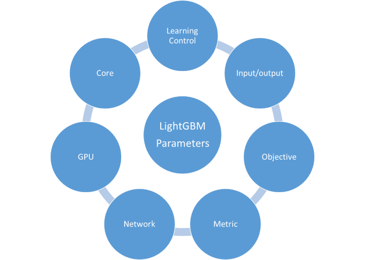
However, we will look at only a few important parameters.

For a more comprehensive list, you can refer to the LightGBM official documentation.

Implementation in Python

Our code here will predict the direction of NIFTY50’s next-day price move (1 or 0) based on a set of input features. The model uses 15 years of historical data.

Installation of LightGBM

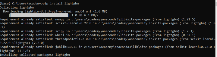
We’ll start with installing the lightGBM package into the Anaconda environment.

This can be done in two ways:

Using the Anaconda prompt

To open Anaconda prompt (Windows) click Start, search for Anaconda Prompt, and click to open. Then simply type in one line of code i.e. "pip install lightgbm". The below screenshot demonstrates the installation.

Using Jupyter notebook

In the jupyter notebook, we can install the lightgbm package using the following line of code "!pip install lightgbm"

!pip install lightgbm

Import the necessary libraries

Download data

We will work with 15 years of daily NIFTY50 data downloaded from Yahoo Finance using the yfinance module. Since we are concerned with only adjusted closing price, we drop the “Close” column from the downloaded data and rename the “Adj Close” column to “AdjClose”

Calculate the parameters

In this step, we calculate the daily returns of NIFTY50 and then create 0,1,2,3,4,5 and 6 period lagged versions of the same which are the input features for the LightGBM model.

Next, we calculate the daily change in price, which will be the target variable(to be predicted by the model). It is calculated as follows:

• If tomorrow’s close price > today’s close price = 1
• If tomorrow’s close price < today’s close price = 0

Define the input features and the output to be predicted

All supervised machine learning models require the input features and the target variable to be defined.

In our case, the input features(lag_0, lag_1, lag_2, lag_3, lag_4, lag_5, lag_6) are stored in X and the target variable in Y(Change).

Split the data into training and testing sets

Next, split the data into train and test datasets(80% - training, 20%-testing)

Create the LightGBM model

Initialise the LightGBM model using LGBMClassifier method with the parameters defined in the code above. Fit the model on 80% of the data, and make predictions on the remaining 20% of the data.

Accuracy results

Output:

Training accuracy: 0.61
Testing accuracy: 0.56

We have now trained the model and made predictions. Let’s examine its accuracy while making predictions. As seen above, the model accuracy is 56%.

Can we use this model for making predictions? Let’s get into the details. We’ll look at the confusion matrix and classification report to better understand the model’s predictability. Since there isn't a significant difference between the training and testing accuracies, we can rule out the case of overfitting.

Plot the confusion matrix for training and testing data

Output:

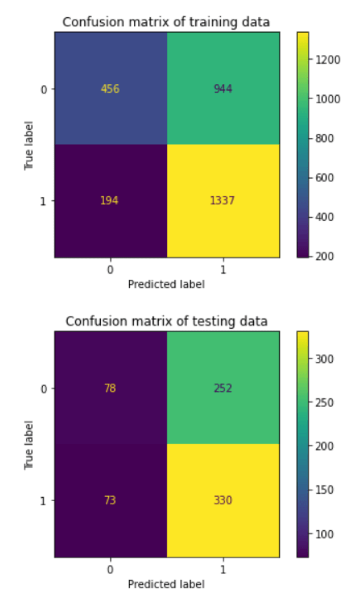
The confusion matrix of testing data tells us that the model has accurately predicted to go long 330 times and inaccurately predicted to go long 252 times. Similarly with the short position you can infer from the above confusion matrix

Classification report

Output:

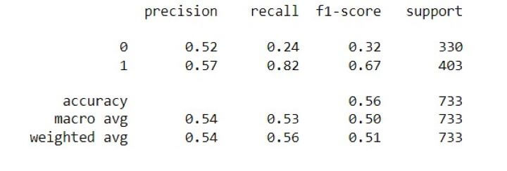
From the above report we can look at f1-score(since it takes into account precision and recall). What does the f1-score tell us? It shows us how many times a model made a correct prediction. It is evident that the f1-score for long positions is higher than short positions. With a few tweaks to the model to improve the accuracy, we could use this model for a long-only strategy.

Feature importance

lgb.plot_importance(model)

Output:

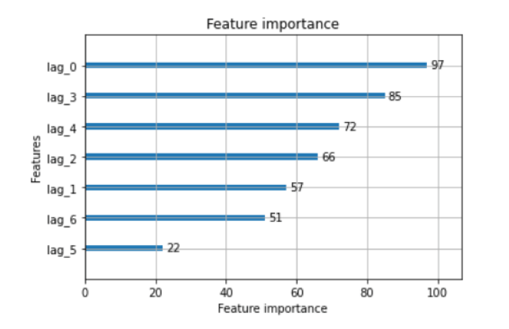
The above plot shows us the importance of each input feature used in the model. It gives a better  insight into the model and helps in dimensionality reduction. For example, some features such as “lag_5” and “lag_6” could be eliminated, since they have low predictive power.

Conclusion

Well, that was a lot of information to digest! So, let us summarise.

In this blog we have understood the basic working principle of LightGBM and how it differs from other gradient-boosting algorithms. We have also seen that LightGBM is indeed faster than its counterpart XGBoost. Finally, we have implemented the LightGBM to the NIFTY50 index and evaluated the model accuracy.

If you would like to venture into the machine learning space and learn more about the various machine learning algorithms and their python implementations. In that case, you can take up the Machine Learning & Deep Learning in Financial Markets course.

Disclaimer: All investments and trading in the stock market involve risk. Any decision to place trades in the financial markets, including trading in stock or options or other financial instruments is a personal decision that should only be made after thorough research, including a personal risk and financial assessment and the engagement of professional assistance to the extent you believe necessary. The trading strategies or related information mentioned in this article is for informational purposes only.