
Have you heard about the Occam’s razor?
To put it simply, William of Ockham stated that, “The simplest solutions are almost always the best solutions.”
But in a post about Naive Bayes, why are we talking about razors? Actually, Naive Bayes implicitly incorporates this belief, because it really is a simple model. Let’s see how a simple model like the Naive Bayes model can be used in trading.
This article covers the following topics:
- What is Naive Bayes?
- Equation for Bayes theorem
- Assumptions of Naive Bayes Model
- Types of Naive Bayes models
- Steps to Build Naive Bayes Model
- Naive Bayes Model in Python
- Advantages of the Naive Bayes model
- Disadvantages of the Naive Bayes model
What is Naive Bayes?
Let’s take a short detour and understand what the “Bayes” in Naive Bayes means. There are basically two schools of thought when it comes to probabilities. One school suggests that the probability of an event can be deduced by calculating the probabilities of all the probable events and then calculating the probability of the event you are interested in.
For example, in the case of coin toss experiment, you know that probability of heads is ½ because there are only two possibilities here, heads or tails.
The other school of thought suggests that probability is more dependent on prior information as well as other factors too. For example, if the probability of a person saying red is their favourite colour is 30% but 50% if they are in love marriage, then your result will be different based on their marital status.
This is known as Bayesian inference, where you try to calculate the probability depending on a certain condition.
And how do you calculate this conditional probability? Let’s see in the next section.
Equation for Bayes theorem
$$P(A|B) = \frac{P(B|A)*P(A)}{P(B)}$$Let’s say A is the event when a person says Red is their favourite colour. Now, let B be the event when the person is married.
Thus, P(A | B) is the likelihood of A saying red is their favourite colour when the person is married.
This is the conditional probability we have to find.
In a similar sense P(B | A) is the likelihood of a person being married when the person says their favourite colour is red.
P(A) and P(B) is the respective probability.
How does this help us in trading?
Let's assume we know the RSI value of a stock.
Now, what if you want to find the probability that the price rises the next day after the RSI goes below 40. Think about it. If the RSI goes below 40 on Tuesday, you will want to buy on Wednesday hoping that price will rise.
This can found by using the Bayes theorem.
Let P(A) be the probability the the price will increase and P(B) be the probability that the RSI was below 40 the previous day.
Now, we will find the probability that the price rises the next day if the RSI is below 40 by the same formula.
Here, B is similar to the feature we define in machine learning. IT can also be called as the evidence.
But hold on! What if we want to check when the RSI is below 40 as well as the “slow k” of stochastic oscillator is more than its “slow d”.
Technically, we can have multiple conditions in Bayes theorem to improve our probability model. If P(C) is the probability that “slow k” passes “slow d”, then the Bayes theorem would be written as,
$$P(A|B,C) = \frac{P(B|A)*P(C|A)*P(A)}{P(B)*P(C)}$$While this looks simple enough to compute, if you add more features to the model, the complexity increases. Here is where the Naive part of the Naive Bayes model comes into the picture.
Assumption of Naive Bayes Model
The Naive bayes model assumes that both B and C are independent events. Further the denominator is also dropped.
This simplifies the model to a great extent and we can simply write the equation as:
P(A|B,C)= P(B|A)*P(C|A)*P(A)
You must remember that this assumption can be incorrect in real life. Logically speaking, both RSI and stochastic indicators are calculated using the same variable, ie price data. Thus, they are not exactly independent.
However, the beauty of NAive Bayes model is that even though this assumption is not true, the model still performs well in various scenarios.
Wait, is there just one type of Naive Bayes model? Actually there are three. Let’s find out in the next section.
Types of Naive Bayes models
Depending on the requirement, you can pick the model accordingly. These models are based on the input data you are working on:
Multinomial: This model is used when we have discrete data and working on its classification. A simple example is we can have the weather (cloudy, sunny, raining) as our input and we want to see in which weather is a tennis match played.
Gaussian: As the name suggests, in this model we work on continuous data which follows a gaussian distribution. An example would be the temperature of the stadium where the match is played.
Binomial: What if we have the input data as simply yes or no, ie a boolean value. In this instance, we will use the binomial model.
The great thing about python is that the sklearn library incorporates all these models. Shall we try to use it for building our own Naive Bayes model? Why not try it out.
Steps to Build Naive Bayes Model
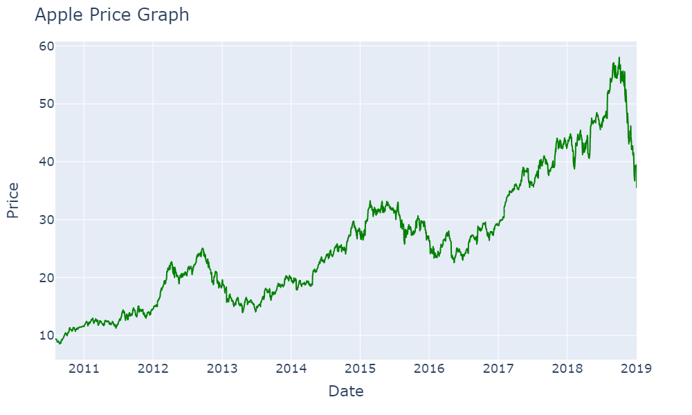
Before we start with the code, we will first try to understand the logic of our exercise. We will be using Apple price data imported from Yahoo Finance and our dataset is from 1 August 2010 to 1 January 2019.
Further, we will use two features.
- RSI Signal - When RSI is less than 40, this variable is set to 1
- Stoch Signal - When the slow k is more than slow d, this variable is set to 1
Finally, our target variable is the next day’s return. If the next day’s return is positive, this is set to 1.
Since we have binary values, we will be using the Binomial Naive Bayes Model in python. Also, bear in mind that this is a long-only strategy but you could modify it to use short signals also. But in that case, you would have to add more rules to the strategy. Let’s see the strategy in action now.
Naive Bayes Model in Python
We will start our strategy by first importing the libraries and the dataset.

We will calculate the indicators as well as their signal values using Talib
To get our target variable, we will calculate our returns and shift by 1 to get the next day’s returns.
We will define the X and y variables for the Naive Bayes model now.
We will now split our dataset into parts, train and test
And now we use the Bernoulli Naive bayes model for binomial analysis.
How was the accuracy of our model. Let’s find out.
Binomial Naive Bayes model accuracy(in %): 51.33333333333333
There is obviously room for improvement here, but this was just a demonstration of how a Naive Bayes model works. But are there special occasions when the model should be used? Let's find out in the next section.
Advantages of the Naive Bayes model
- The main advantage of the Naive bayes model is its simplicity and fast computation time. This is mainly due to its strong assumption that all events are independent of each other
- They can work on limited data as well
- Their fast computation is leveraged in real time analysis when quick responses are required
Although this speed comes at a price. Let’s find out how in the next section.
Disadvantages of Naive Bayes Model
- Since Naive Bayes assumes that all events are independent of each other, it cannot compute the relationship between the two events
- The Naive Bayes Model is fast but it comes at the cost of accuracy. NAive Bayes is sometimes called bad estimator
- The equation for Naive Bayes shows that we are multiplying the various probabilities. Thus, if one feature returned 0 probability, it could turn the whole result as 0. There are however, various methods to overcome this instance. One of the more famous ones is called Laplace correction. In this method, the features are combined or the probability is set to 1 which ensures that we do not get zero probability.
Conclusion
The Naive Bayes model, despite the fact that it is naive, is pretty simple and effective in a large number of use cases in real life. While it is mostly used for text analysis, it has been used as a verification tool in the field of trading.
The Naive Bayes model can also be used as a stepping stone towards more precise and complex classification based machine learning models. You can check out the course on Trading with Machine Learning: Classification and SVM to incorporate various ML models in your trading arsenal.
Disclaimer: The views, opinions, and information provided within this guest post are those of the author alone and do not represent those of QuantInsti®. The accuracy, completeness, and validity of any statements made or the links shared within this article are not guaranteed. We accept no liability for any errors, omissions or representations. Any liability with regards to infringement of intellectual property rights remains with them.
