Machine Learning for Algorithmic Trading in Python: A Complete Guide

By Chainika Thakar and Varun Divakar

If you've been curious about leveraging Machine Learning for algorithmic trading with Python, you're joining a growing trend in the financial industry. Machine learning has gained significant popularity among quant firms and hedge funds in recent years. These entities have recognised the potential of machine learning for algorithmic trading.

While specific algorithmic trading strategies employed by quant hedge funds are typically proprietary and kept confidential, it is widely acknowledged that many top funds heavily rely on machine learning techniques.

For instance, Man Group's AHL Dimension program, a hedge fund managing over $5.1 billion, incorporates AI and machine learning in its trading operations. Taaffeite Capital, another notable example, proudly claims to trade fully systematically and automatically using proprietary machine learning systems.

In this Python machine learning tutorial, we aim to explore how machine learning has transformed the world of trading. We can develop machine-learning  algorithms to make predictions and inform trading decisions by harnessing the power of Python and its diverse libraries. While the tutorial will not reveal specific hedge fund strategies, it will guide you through the process of creating a simple Python machine-learning algorithm to predict the closing price of a stock for the following day.

By understanding the fundamentals of machine learning, Python programming, financial markets, and statistical concepts, you can unlock opportunities for algorithmic trading using machine learning in Python. From acquiring and preprocessing data to creating hyperparameters, splitting data for evaluation, optimising model parameters, making predictions, and assessing performance, you will gain insights into the entire process. Get ahead with the best Algorithmic Trading books available.

This guide to algo for trading emphasizes the importance of mastering key areas such as machine learning, Python programming, and financial market analysis to effectively use machine learning in trading strategies. Understanding the complete workflow, from data preprocessing to performance evaluation, is essential for building and optimizing trading algorithms.

When exploring algo trading for beginners, it’s helpful to break down each step methodically. Starting with basic concepts like data preprocessing and gradually advancing to model optimization ensures a solid foundation. This structured approach makes navigating the complexities of algorithmic trading smoother and more manageable.

It's important to note that using machine learning in algorithmic trading has its pros and cons.

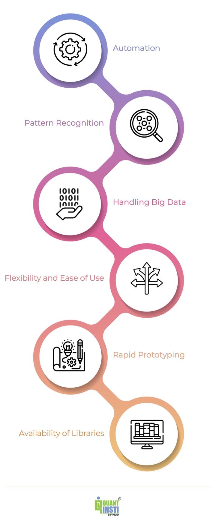
On the positive side, it offers automation, pattern recognition, and the ability to handle large and complex datasets. However, challenges such as model complexity, the risk of overfitting, and the need to adapt to dynamic market conditions should be taken into account.

By embarking on this journey of using machine learning in Python for algorithmic trading, you will gain valuable knowledge and skills to apply in finance and explore the exciting intersection of data science and trading.

All the concepts covered in this blog are taken from this Quantra course on Python for Machine Learning in Finance.

This blog covers:

• How machine learning gained popularity?
• Why use machine learning with Python in algorithmic trading?
• Prerequisites for creating machine learning algorithms for trading using Python
• How to use algorithmic trading with machine learning in Python?
• Getting the data and making it usable for machine learning algorithm
• Creating hyperparameters
• Splitting the data into test and train sets
• Getting the best-fit parameters to create a new function
• Making the predictions and checking the performance
• Comparing pros and cons of using machine learning with Python for algorithmic trading
• FAQs

How machine learning gained popularity?

Machine learning packages and libraries are developed either in-house by firms for proprietary use or by third-party developers who make them freely available to the user community. The availability of these packages has significantly increased in recent years, empowering developers to access a wide range of machine-learning techniques for their trading needs.

There are numerous machine learning algorithms, each classified based on its functionality. For example, regression algorithms model the relationship between variables, while decision tree algorithms construct decision models for classification or regression problems. Among quants, certain algorithms have gained popularity, such as

• Linear Regression
• Logistic Regression
• Random Forests (RM)
• Support Vector Machine (SVM)
• K-Nearest Neighbor (kNN) Classification and
• Regression Tree (CART) Deep Learning

These Machine Learning algorithms for trading are used by trading firms for various purposes including:

• Analysing historical market behaviour using large data sets
• Determine optimal inputs (predictors) to a strategy
• Determining the optimal set of strategy parameters
• Making trade predictions etc.

Why use machine learning with Python in algorithmic trading?

Thanks to its active and supportive community, Python for trading has gained immense popularity among programmers. According to Stack Overflow's 2020 Developer Survey, Python ranked as the top language for the fourth consecutive year, with developers expressing a strong desire to learn it. Python's dominance in the developer community makes it a natural choice for trading, particularly in the quantitative finance field.

To enhance your skills in this area, consider enrolling in quantitative trading courses that focus on leveraging Python and machine learning techniques for effective algorithmic trading strategies.

Python's success in trading is attributed to its scientific libraries like Pandas, NumPy, PyAlgoTrade, and Pybacktest, which enable the creation of sophisticated statistical models with ease. The continuous updates and contributions from the developer community ensure that Python trading libraries remain relevant and cutting-edge. Additionally, there is the availability of libraries like

• Pandas
• NumPy
• PyAlgoTrade and more.

Coming to machine learning with python, there are several reasons why machine learning with Python is widely used in algorithmic trading:

Moreover, you can check out this informative video below to find out how machine learning for algorithmic trading works.

Prerequisites for creating machine learning algorithms for trading using Python

Extensive Python libraries and frameworks make it a popular choice for machine learning tasks, enabling developers to implement and experiment with various algorithms, process and analyse data efficiently, and build predictive models.

In order to create the machine learning algorithms for trading using Python, you will need the following prerequisites:

• Installation of Python packages and libraries meant for machine learning
• Full-fledged knowledge of steps of machine learning
• Knowing the application models

Install a few packages and libraries

Python machine learning specifically focuses on using Python for the development and application of machine learning models.

You may add one line to install the packages “pip install numpy” You can install the necessary packages in the Anaconda Prompt using the codes as mentioned below.

• Scikit-learn for machine learning
• TensorFlow for deep learning
• Keras for deep learning
• PyTorch for neural networks
• NLTK for natural language processing

Full-fledged knowledge of steps of machine learning

In addition to general Python knowledge, proficiency in Python machine learning necessitates a deeper understanding of machine learning concepts, algorithms, model evaluation, feature engineering, and data preprocessing.

Knowing the application models

The primary focus of Python machine learning is the development and application of models and algorithms for tasks like classification, regression, clustering, recommendation systems, natural language processing, image recognition, and other machine learning applications.

How to use algorithmic trading with machine learning in Python?

Let us see the steps to doing algorithmic trading with machine learning in Python. These steps are:

• Problem statement
• Getting the data and making it usable for machine learning algorithm
• Creating hyperparameter
• Splitting the data into test and train sets
• Getting the best-fit parameters to create a new function
• Making the predictions and checking the performance

Problem Statement

Let’s start by understanding what we are aiming to do. By the end of this machine learning for algorithmic trading with Python tutorial, I will show you how to create an algorithm that can predict the closing price of a day from the previous OHLC (Open, High, Low, Close) data.

I also want to monitor the prediction error along with the size of the input data.

Let us import all the libraries and packages needed to build this machine-learning algorithm.

Getting the data and making it usable for machine learning algorithm

To create any algorithm, we need data to train the algorithm and then to make predictions on new unseen data. In this machine learning for algorithmic trading with Python tutorial, we will fetch the data from Yahoo.

To accomplish this, we will use the data reader function from the pandas library. This function is extensively used, enabling you to get data from many online sources.

We are fetching the data of AAPL(ticker) or APPLE. This stock can be used as a proxy for the performance of the S&P 500 index. We specify the year starting from which we will be pulling the data.

Once the data is in, we will discard any data other than the OHLC, such as volume and adjusted Close, to create our data frame ‘df ’.

Now we need to make our predictions from past data, and these past features will aid the machine learning model trade. So, let's create new columns in the data frame that contain data with one day lag.

Incorporating AI in trading enhances our predictive capabilities by analyzing historical data patterns more effectively, enabling us to refine our trading strategies based on insights derived from past performance.

Note: The capital letters are dropped for lower-case letters in the names of new columns.

Creating Hyperparameters

Although the concept of hyperparameters  is worthy of a blog in itself, for now I will just say a few words about them. These are the parameters that the machine learning algorithm can’t learn over but needs to be iterated over. We use them to see which predefined functions or parameters yield the best-fit  function.

In this example, I have used Lasso regression which uses the L1 type of regularisation. This is a type of machine learning model based on regression analysis which is used to predict continuous data.

This type of regularisation is very useful when you are using feature selection. It is capable of reducing the coefficient values to zero. The SimpleImputer function replaces any NaN values that can affect our predictions with mean values, as specified in the code.

The ‘steps’ are a bunch of functions that are incorporated as a part of the Pipeline function. The pipeline is a very efficient tool to carry out multiple operations on the data set. Here we have also passed the Lasso function parameters along with a list of values that can be iterated over.

Although I am not going into details of what exactly these parameters do, they are something worthy of digging deeper into. Finally, I called the randomised search function for performing the cross-validation.

In this example, we used 5-fold cross-validation. In k-fold cross-validation, the original sample is randomly partitioned into k equal-sized subsamples. Of the k subsamples, a single subsample is retained as the validation data for testing the model, and the remaining k-1 subsamples are used as training data.

The cross-validation process is then repeated k times (the folds), with each of the k subsamples used exactly once as the validation data. Cross-validation combines (averages) measures of fit (prediction error) to derive a more accurate estimate of model prediction performance.

Based on the fit parameter, we decide on the best features.

In the next section of the machine learning for algorithmic trading with Python tutorial, we will look at test and train sets.

Splitting the data into test and train sets

First, let us split the data into the input values and the prediction values. Here we pass on the OHLC data with one day lag as the data frame X and the Close values of the current day as y. Note the column names below in lower-case.

In this example, to keep the machine learning for algorithmic trading with Python tutorial short and relevant, I have chosen not to create any polynomial features but to use only the raw data.

If you are interested in various combinations of the input parameters and with higher degree polynomial features, you are free to transform the data using the PolynomialFeature() function from the preprocessing package of scikit learn.

You can find detailed information in Quantra course on Python for Machine Learning in Finance.

Now, let us also create a dictionary that holds the size of the train data set and its corresponding average prediction error.

Getting the best-fit parameters to create a new function

I want to measure the performance of the regression function as compared to the size of the input dataset. In other words, I want to see if, by increasing the input data, we will be able to reduce the error. For this, I used for loop to iterate over the same data set but with different lengths.

At this point, I would like to add that for those of you who are interested, explore the ‘reset’ function and how it will help us make a more reliable prediction.

(Hint: It is a part of the Python magic commands)

Let me explain what I did in a few steps.

First, I created a set of periodic numbers ‘t’ starting from 50 to 97, in steps of 3. The purpose of these numbers is to choose the percentage size of the dataset that will be used as the train data set.

Second, for a given value of ‘t’, I split the length of the data set to the nearest integer corresponding to this percentage. Then I divided the total data into train data, which includes the data from the beginning till the split, and test data, which includes the data from the split till the end. The reason for adopting this approach and not using the random split is to maintain the continuity of the time series.

After this, we pull the best parameters that generated the lowest cross-validation error and then use these parameters to create a new reg1 function, a simple Lasso regression fit with the best parameters.

Making the predictions and checking the performance

Now let us predict the future close values. To do this, we pass on test X, containing data from split to end, to the regression function using the predict() function. We also want to see how well the function has performed, so let us save these values in a new column.

As you might have noticed, I created a new error column to save the absolute error values. Then I took the mean of the absolute error values, which I saved in the dictionary we had created earlier.

Now it's time to plot and see what we got.

I created a new Range value to hold the average daily trading range of the data. It is a metric I would like to compare with when making a prediction. The logic behind this comparison is that if my prediction error is more than the day’s range, then it is likely that it will not be useful.

I might as well use the previous day’s High or Low as the prediction, which will turn out to be more accurate.

Please note I have used the split value outside the loop. This implies that the average range of the day you see here is relevant to the last iteration.

Let’s execute the code and see what we get.

Output:

dict_values([0.016572107043186714, 0.016153385252750785, 0.01588065955869017, 0.015618964962728854, 0.015590553449790096, 0.015309647511941773, 0.01493713896774542, 0.014651947116887016, 0.014501339871063298, 0.014370132121548317, 0.014384337806316318, 0.014279892175630736, 0.014518721712207314, 0.014650203218479405, 0.014598423460738174, 0.014489723845538215])

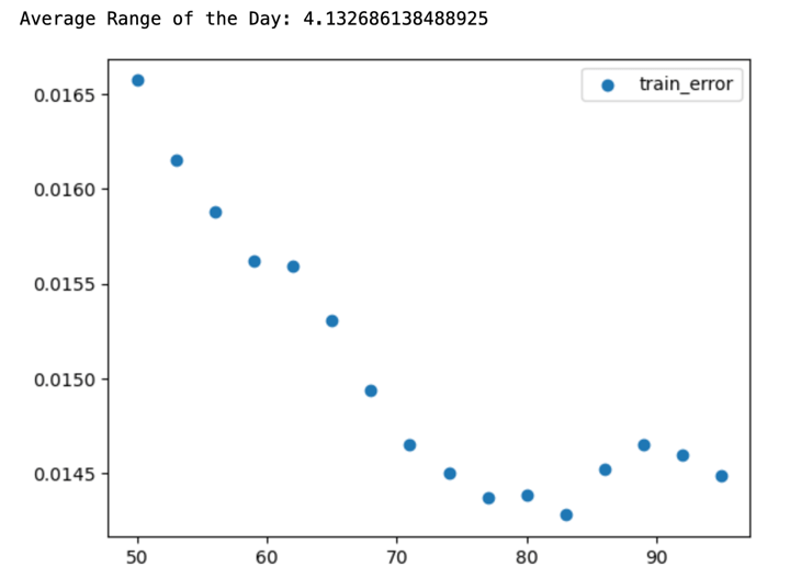
Some food for thought.

What does this scatter plot tell you? Let me ask you a few questions.

• Is the equation over-fitting?
• The performance of the data improved remarkably as the train data set size increased. Does this mean if we give more data, the error will reduce further?
• Is there an inherent trend in the market, allowing us to make better predictions as the data set size increases?
• Last but the best question: How will we use these predictions to create a trading strategy?

FAQs

At the end of the last section of the tutorial Machine Learning algorithms for Trading, I asked a few questions. Now, I will answer them all at the same time. I will also discuss a way to detect the regime/trend in the market without training the algorithm for trends.

You can read more about 5 Things to know before starting Algorithmic Trading

But before we go ahead, please use a fix to fetch the data from Yahoo Finance to run the code below.

Let’s start with the questions now, shall we?

Q: Is the equation over-fitting?
A: This was the first question I had asked. To know if your data is overfitting or not, the best way to test it would be to check the prediction error that the algorithm makes in the train and test data.

To do this, we will have to add a small piece of code to the already written code.

Second, if we run this piece of code, then the output would look something like this.

Output:

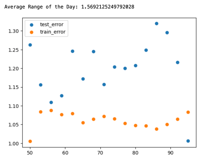
Our algorithm is doing better in the test data compared to the train data. This observation in itself is a red flag. There are a few reasons why our test data error could be better than the train data error:

1. If the train data had greater volatility (Daily range) compared to the test set, then the prediction would also exhibit greater volatility.
2. If there was an inherent trend in the market that helped the algo make better predictions.

Now, let us check which of these cases is true. If the range of the test data was less than the train data, then the error should have decreased after passing more than 80% of the data as a train set, but it increases.

Next, to check if there was a trend, let us pass more data from a different time period.

If we run the code, the result would look like this:

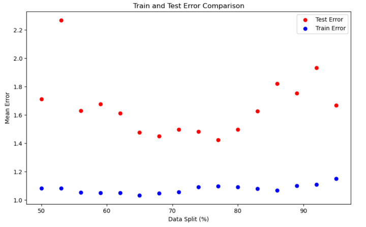
So, giving more data did not make your algorithm work better, but it made it worse. In time-series data, the inherent trend plays a very important role in the algorithm's performance on the test data.

As we saw above it can yield better than expected results sometimes. Our algo was doing so well because the test data was sticking to the main pattern observed in the train data.

So, if our algorithm can detect the underlying trend and use a strategy for that trend, then it should give better results. I will explain this in more detail below.

Q: Can the machine learning algorithm detect the inherent trend or market phase (bull/bear/sideways/breakout/panic)?

Q: Can the database be trimmed to train different algos for different situations?

A: The answer to both the questions is YES!

We can divide the market into different regimes and then use these signals to trim the data and train different algorithms for these datasets. To achieve this, I choose to use an unsupervised machine learning algorithm. Explore the 'unsupervised learning course' from Quantra.

From here on, this machine learning for algorithmic trading with Python tutorial will be dedicated to creating an algorithm that can detect the inherent trend in the market without explicitly training for it.

First, let us import the necessary libraries.

Then we fetch the OHLC data from Google and shift it by one day to train the algorithm only on the past data.

Next, we will instantiate an unsupervised machine learning algorithm using the ‘Gaussian mixture’ model from sklearn.

In the above code, I created an unsupervised-algo that will divide the market into 4 regimes, based on the criterion of its choosing. We have not provided any training dataset with labels like in the previous section of the Python machine learning tutorial.

Next, we will fit the data and predict the regimes. Then we will store these regime predictions in a new variable called regime.

Then, create a dataframe called Regimes which will have the OHLC and Return values along with the corresponding regime classification.

After this, let us create a list called ‘order’ that has the values corresponding to the regime classification, and then plot these values to see how well the algo has classified.

The final regime differentiation would look like this:

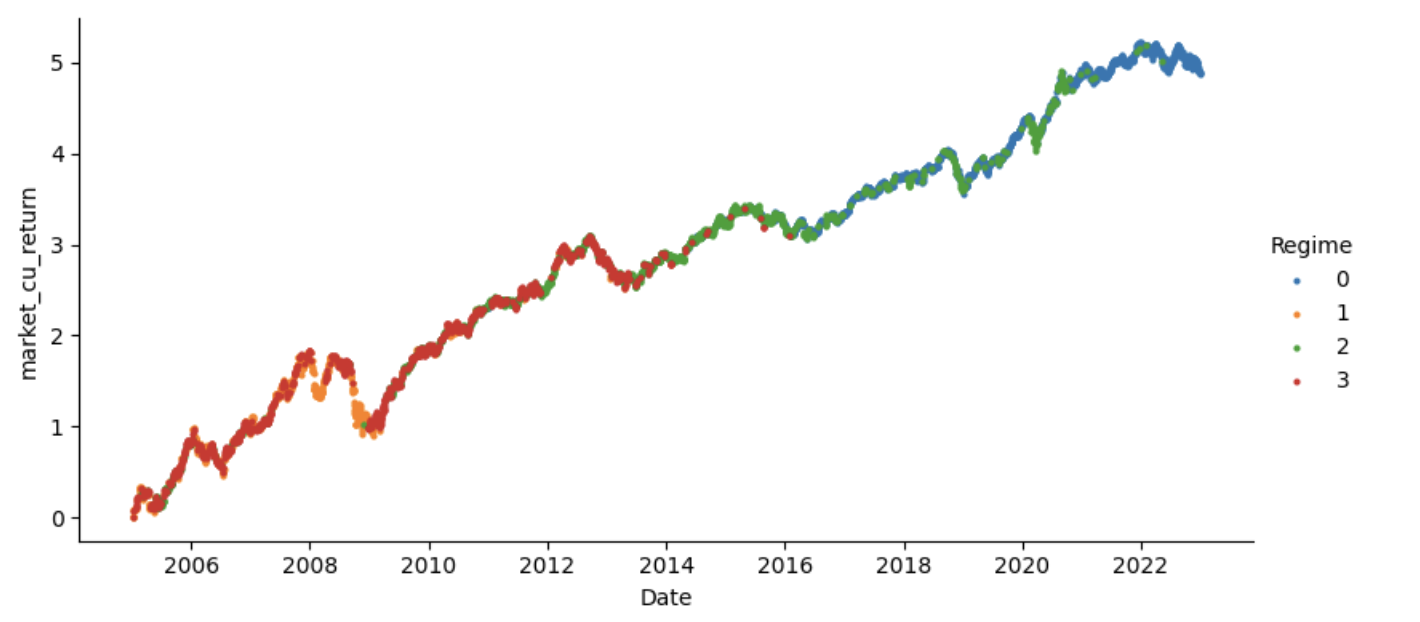
This graph looks pretty good to me. We can conclude a few things by looking at the chart without actually looking at the factors based on which the classification was done.

1. The red zone is the low volatility or the sideways zone
2. The orange zone is a high volatility zone or panic zone.
3. The blue zone is a breakout zone.
4. The green zone: Not entirely sure but let us find out.

Use the code below to print the relevant data for each regime.

The output would look like this:

Mean for regime 0: 75.93759504542675

Co-Variance For regime 0: 189860766854172.0

Mean for regime 1: 4.574220463352975

Co-Variance For regime 1: 3.1775040099630092e+16

Mean for regime 2: 21.598410250495476

Co-Variance For regime 2: 1583756227241176.8

Mean for regime 3: 7.180175568961408

Co-Variance For regime 3: 2432345114794574.0

The data can be inferred as follows:

1. Regime 0: Low mean and High covariance.
2. Regime 1: High mean and High covariance.
3. Regime 2: High mean and Low covariance.
4. Regime 3: Low mean and Low covariance.

So far, we have seen how to split the market into various regimes.

But the question of implementing a successful strategy is still unanswered. If you want to learn how to code a machine learning trading strategy then your choice is simple:

To rephrase Morpheus from the Matrix movie trilogy,

This is your last chance. After this, there is no turning back.

You take the blue pill—the story ends, you wake up in your bed and believe that you can trade manually.

You take the red pill—you stay in the Algoland, and I show you how deep the rabbit hole goes.

Remember: All I'm offering is the truth. Nothing more.

A step further into the world of Machine Learning algorithms for Trading

Keeping oneself updated is of prime importance in today’s world. Having a learner’s mindset always helps to enhance your career and pick up skills and additional tools in the development of trading strategies for themselves or their firms.

Here are a few books which might be interesting:

1. Gareth James, Daniela Witten, Trevor Hastie and Robert Tibshirani Introduction to statistical learning
2. The Hundred-Page Machine Learning Book by Andriy Burkov
3. Hastie, Tibshirani, and Friedman's The Elements of Statistical Learning

Comparing pros and cons of using machine learning with Python for algorithmic trading

Let us now compare the pros and cons of using machine learning with Python for algorithmic trading below:

Bibliography

1. A Machine Learning Stock Trading Strategy Using Python
2. Algorithmic Trading in Python with Machine Learning: Walkforward Analysis

Conclusion

Overall, we have gone through the entire journey of how you can learn to create and use your very own machine learning models in Python, using various examples. The entire process is explained with the help of Python codes that will be helpful in your practice as well.

If you have any comments or suggestions about this article, please share them with us in the comments below.

If you wish to create trading strategies and understand the limitations of your models, check out this course on  Python for Machine Learning in Finance. This course will guide you through algo trading programming, helping you evaluate the performance of machine learning algorithms and perform backtesting, paper trading, and live trading with Quantra’s integrated learning.

Note: The original post has been revamped on 18th August 2023 for accuracy, and recentness.

Disclaimer: All data and information provided in this article are for informational purposes only. QuantInsti^® makes no representations as to accuracy, completeness, currentness, suitability, or validity of any information in this article and will not be liable for any errors, omissions, or delays in this information or any losses, injuries, or damages arising from its display or use. All information is provided on an as-is basis.