By José Carlos Gonzáles Tanaka
Whenever you want to estimate a model for multiple time series, the Vector Autoregression (VAR) model will serve you well. This model is suitable for handling multiple time series in a single model. You will learn here the theory, the intricacies, the issues and the implementation in Python and R.
- What is a VAR model?
- Creating a VAR model
- A stationary VAR
- VAR Lag Selection Criteria
- Estimation of a VAR in Python
- Estimation of a VAR in R
- An equally-weighted portfolio using VAR in Python and R
- Considerations while estimating a VAR model
What is a VAR model?
Let’s remember what is an ARMA model. An ARMA(p,q) model is an autoregressive moving average model applied to a single time series. The single-equation model can be mathematically formulated as
$$y_{t}=\phi_1 y_{t-1}+\phi_2 y_{t-2} + ... + \phi_p y_{t-p}+\epsilon+\theta_1\epsilon_{t-1}+\theta_2\epsilon_{t-2}+ ... + \theta_q\epsilon_{t-q}$$Whenever you want to model a time series with its own series, you can use this model. In case you want to estimate this model with only the autoregressive component, you can do something like the following
$$y_{t}=\phi_1 y_{t-1}+\phi_2 y_{t-2} + ... + \phi_p y_{t-p}+\epsilon$$Which is nothing but an AR(p) model. What about if we estimate this model for two time series?
Well, we can surely do it. Let’s write this as
$$y_{t}=\phi_{y1} y_{t-1}+\phi_{y2} y_{t-2} + ... + \phi_{yp} y_{t-p}+\epsilon$$ $$x_{t}=\phi_{x1} x_{t-1}+\phi_{x2} x_{t-2} + ... + \phi_{xp} x_{t-p}+\epsilon$$We can estimate these two models separately for each time series. However, we can also do it together!
Creating a VAR model
Let’s create first a bivariate VAR(1) model. The math equations will look something like this
$$Y_{1,t}=\phi_{11} Y_{1,t-1}+\phi_{12} Y_{2,t-1} +\epsilon_{1,t}$$ $$Y_{2,t}=\phi_{21} Y_{1,t-1}+\phi_{22} Y_{2,t-1} +\epsilon_{2,t}$$We can think of this model in terms of matrices, like as follows:
$$Y_t= \Phi Y_{t-1}+\mathcal{E}_t$$Where
\(Y_t = \begin{bmatrix} Y_{1,t} \\ Y_{2,t}\end{bmatrix}\)\(\Phi = \begin{bmatrix} \phi_{11} & \phi_{12}\\ \phi_{21} & \phi_{22}\end{bmatrix}\)
\(Y_{t-1} = \begin{bmatrix} Y_{1,t-1} \\ Y_{2,t-1}\end{bmatrix}\)
\(\mathcal{E}_t = \begin{bmatrix} \epsilon_{1,t} \\ \epsilon_{2,t}\end{bmatrix}\)
To sum up:
- First, it’s bivariate because we have two time series.
- It’s VAR(1) because we only have one lag for each time series. Also, note that we have the first lag of each time series on each time series equation.
- Each time series equation has its own error component
- We have four parameters which have their specific notation due to the fact that while estimating, you will find that each parameter will have its unique value.
Time Series Analysis
Financial Time Series Analysis for Smarter Trading
A stationary VAR
Before you start estimating the equation, let me tell you that, as well as for an ARMA model, there’s a need to have a stable VAR, i.e., a stationary VAR model.
How do you check for stationarity in this model? Well, usually practitioners find the order of integration of each time series separately. So you need to do the following:
- Apply, e.g., an ADF to each time series separately.
- Find for each time series its “d” order of integration.
- Difference the time series as per its corresponding “d” order of integration.
- Use the differenced data to estimate your VAR model.
VAR Lag Selection Criteria
Usually, when estimating this model, you will ask yourself: How many lags should I apply for each time series?
The question is wrongly formulated. You should actually ask: How many lags should I apply for the model?
Practitioners usually estimate the autoregressive lag for the whole model, without considering a specific “p” for each time series. Please, also take into account that, while getting the VAR output results, you shouldn’t worry too much about the significance of each parameter in the model.
You’re better off concentrating on the predictive power than on the specifics of the significance of each variable in the model.
Coming back to our original question, how many lags we should apply can be answered as follows:
- Estimate a VAR model with different lags.
- Save the information criteria of your preference for each VAR model.
- Choose the model with the lowest information criteria.
Fortunately, Python and R have inside their libraries the computation of this process automatically so we don’t need to do this through a for loop.
Estimation of a VAR in Python
Let’s estimate a VAR model. First we find the order of integration of each time series. We make the following steps:
- Step 1: Import the necessary libraries
- Step 2: Import the data
- Step 3: Create first and second differences of each time series
- Step 4: Identify the order of integration of each stock.
- Step 5: Output a table to show the order of integration for each asset.
- Step 6: Estimate a VAR
Step 1: Import the necessary libraries
Step 2: Import the data
We’re going to download price data from 2000 to September 2023 of 7 stocks: Microsoft, Apple, Tesla, Netflix, Meta (ex-Facebook), Amazon and Google. We will use the Yahoo finance API.
Next, as we previously said, we need to have the VAR stationary. To have that, we need to have stationary time series. We apply an ADF test to each stock price. In case they’re not stationary, we apply the same ADF test but to its first difference.
Grasping the concept of Stationary Time Series is essential for ensuring accurate results in your analysis. By confirming stationarity through tests like ADF, you set the stage for reliable forecasting and robust models. Explore further to see how this step can refine your approach and enhance the effectiveness of your time series analysis.
In case this first difference is not stationary, we apply the ADF test to the second difference and so on until we find the order of integration. Throughout all this, we create a dataframe to save all the p-values of the tests applied to each asset.
Step 3: Create first and second differences of each time series
Step 4: Identify the order of integration of each stock.
In the second loop we compute the ADF test and extract the p-value. As you can see, we apply auto_lag = ‘aic’, which means we identify the autoregressive lag order of the ADF regression automatically with the help of the Akaike information criteria.
Besides we use a constant for the ADF in price levels since each asset has a trend, and for the first and second differences we don’t add a constant or a trend since these two time series don’t present a mean different from zero.
Step 5: Output a table to show the order of integration for each asset.
Let’s see the results in the table:
| prices_pvalue | dif_pvalue | dif2_pvalue | Integration_order | |
| MSFT | 0.954707 | 0 | 0 | 1 |
| AAPL | 0.940228 | 0 | 0 | 1 |
| TSLA | 0.657697 | 0 | 0 | 1 |
| NFLX | 0.582101 | 0 | 0 | 1 |
| META | 0.497799 | 0 | 0 | 1 |
| AMZN | 0.70171 | 0 | 0 | 1 |
| GOOGL | 0.781121 | 0 | 0 | 1 |
As you can see, the order of integration of each asset price is 1. Consequently, we need to use the first difference of each variable to estimate the VAR.
Step 6: Estimate a VAR
Let’s estimate a simple VAR(1) model. First, we create the “var” data. We get the first log difference and drop the NaN values.
We ended up with 2844 observations for each asset. We proceed to estimate the VAR.
Inside the fit parenthesis, we code 1, meaning we are going to create a VAR with one lag for each time series.
In the summary output, you will see the parameters for the lag of each time series. As we told you previously, you don’t need to worry about the significance of each of them, as long as you are sure the model provide good forecasts.
Estimation of a VAR in R
We proceed to teach how to do it in R. We already know the order of integration of each time series, so we continue with the rest of the steps:
- Step 1: Install and import the necessary libraries.
- Step 2: Import the data.
- Step 3: Create a dataframe to put together the adjusted close prices of each asset.
- Step 4: Create the returns dataframe.
- Step 5: Select the best lag order based on the BIC.
- Step 6: Estimate a VAR with the best lag order.
- Step 7: Forecast the next day’s assets’ return.
Step 1: Install and import the necessary libraries
Step 2: Import the data
Then we download the same data for the same span and save it in the “df” environment.
Then, we create a dataframe called “df2” to save all the stock prices. We do this since the “df” environment has each stock data separately.
Step 3: Create a dataframe to put together the adjusted close prices of each asset
We then create a stock price returns dataframe called “var_data”. We use log returns.
Step 4: Create the returns dataframe
We then create a dataframe called data to save only the returns data and deselect the date column. Next, we proceed to select the best lag order for the VAR model using the VARselect method.
We assign “none” to type, i.e., we don’t add a constant nor a trend. We choose the best lag based on the Bayesian information criteria. Finally, we output the summary results.
The last date in the dataframe is 2023-09-09. We proceed to forecast the next trading day’s returns with
Step 7: Forecast the next day’s assets’ return
In case we want to forecast the next 2 trading days’ returns, we would change n.ahead to 2, and so on.
An equally-weighted portfolio using VAR in Python and R
Can we create this type of portfolio with VAR forecasts?
Of course, we can. Using the same libraries from before, we use again the “var_data” dataframe. For each day, we will be doing the following:
- Use the previous 1000 days’ returns as input for the VAR model.
- We fit up to 20-lag VARs and select the model with the lowest AIC.
- Forecast the next day’s returns
- In case the estimation doesn’t work we assign 0 to the forecast columns, i.e., we take no position at all on all the stocks.
- Go long for each stock whenever its forecasted return is positive, otherwise, we take no position at all on the stock.
- Create an equally-weighted portfolio with the stocks which have a long signal for that day.
We follow the next steps:
- Step 1: Let’s define first our variables.
- Step 2: Decide to make forecasts from 2019-01-01 onwards.
- Step 3: Create a dataframe to have 1002 days to forecast each stock price return.
- Step 4: Run a loop to estimate the best VAR on each day and forecast each asset’s price return.
- Step 5: Create the VAR-based strategy signals.
- Step 6: Create the benchmark portfolio cumulative returns.
- Step 7: Create the VAR-based strategy cumulative returns.
- Step 8: Graph both portfolios.
- Step 9: Output some summary statistics metrics for each portfolio and compare.
Let's begin!
Step 1: Let’s define first our variables.
Step 2: Decide to make forecasts from 2019-01-01 onwards.
Step 3: Create a dataframe to have 1180 days to forecast each stock price return.
On the above code, we create a “models” dictionary to save the VAR object and its results. Then, we create the variable “initial_iloc_to_forecast” to get the data position number in which the var_data date “2019-01-01” is located.
Next, we set the span of the input data to be 1000. We create another dataframe in which we will save the forecast results named “df_results”. We set the stock forecast default values to zero. Additionally, we create a “forecast_span” range which will be used for the below loop.
Step 4: Run a loop to estimate the best VAR on each day and forecast each asset’s price return.
Let’s show the for loop we will use to create the VAR forecasts
for i in range(total_no_of_forecasts):
For each day, we use a try-except block. In case the VAR estimation doesn’t occur, we set the forecast values to zero so we don’t take a position on the stocks. In case we can estimate, we create a VAR object with the selected data which will be the previous 1000 days’ observations.
We proceed to estimate up to the 20-lag VAR and select the best model with the Akaike information criteria. We save the best lag order in “lag_order” and use it to forecast the next day’s returns.
Finally, we empty the “models” dictionary so it can be used for the next day's estimation.
Step 5: Create the VAR-based strategy signals
Next we create the signals. For each stock, we will go long whenever the forecast return is positive. We take no position when the return is negative.
Step 6: Create the benchmark portfolio cumulative returns.
Then, we create the buy-and-hold cumulative returns together with the VAR-based strategy cumulative returns
Step 7: Create the VAR-based strategy cumulative returns.
Step 8: Graph both portfolios
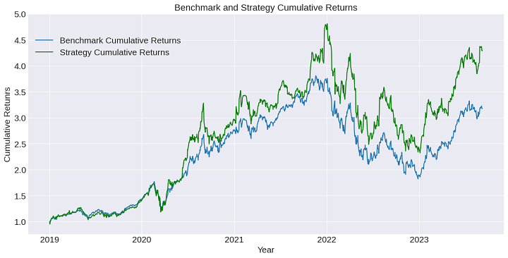
Next, we plot both cumulative returns
Let’s see the graph:
Step 9: Output some summary statistics metrics for each portfolio and compare.
Let’s use pyfolio to create some basic statistics
In the following table, we present the sumup of both portfolio returns
Statistic
| Statistic | Benchmark Portfolio | Strategy Portfolio |
| Annual return | 28.1% | 37.0% |
| Cumulative returns | 218.3% | 336.4% |
| Annual volatility | 31.9% | 36.4% |
| Sharpe ratio | 0.94 | 1.05 |
| Maximum drawdown | 52.2% | 51.7% |
| Calmar ratio | 0.54 | 0.72 |
| Sortino ratio | 1.32 | 1.52 |
There are some insights we can get from this graph and table:
- The strategy cumulative returns outperforms the benchmark.
- Even though the volatility for the strategy, we have a higher Sharpe ratio.
- Calmar ratio and Sortino ratios are higher for the strategy, i.e., even though we have a higher volatility in the strategy, the strategy outperforms in most of the statistics to the benchmark.
Check the same code in R. The span was changed to 1500 to see how the portfolio returns change. We use the same libraries from before and also the same var_data created.
We start forecasting on 2019-01-01. In this case, we estimate up to the 15-lag VAR and choose the best model as per the Bayesian Information criteria.
The code is the following:
The daily forecast loop and the strategy returns computations are presented in the following code snippet.
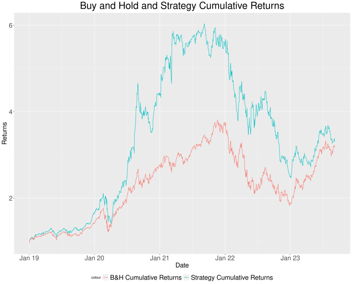
Let’s check the graph:
Let’s sum up the summary statistics in a table:
| Statistic | Benchmark Portfolio | Strategy Portfolio |
| Annual return | 28.1% | 29.2% |
| Cumulative returns | 218.3% | 231.5% |
| Annual volatility | 31.9% | 35.7% |
| Sharpe ratio | 0.94 | 0.89 |
| Maximum drawdown | 52.2% | 59.0% |
| Calmar ratio | 0.54 | 0.49 |
| Sortino ratio | 1.32 | 1.51 |
Some suggestions:
- The strategy risk metrics result higher than the 1000-span VAR strategy, although it also outperforms the benchmark in the majority of the statistics.
- We should optimize the span in order to improve the performance.
- We have used up to 20 lags to create the VAR models. This might be too much, there might be models with unit roots values not too convenient for the VAR stability. You can decrease the maximum number of lags.
- It seems that the VAR model performs well when assets are bullish. We might improve the performance if we control for the bearish scenario with a moving average signal.
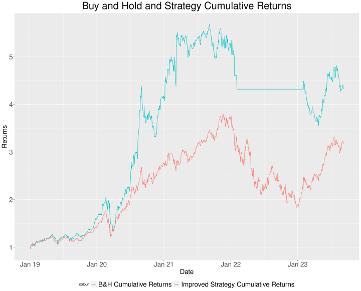
Let’s try the last suggestion in R. We create a 200-day moving average signal with the following rule:
- If the buy-and-hold cumulative returns is higher than its 200-day moving average, then we use the VAR-based long signal if available.
- Otherwise, we take no position at all.
This signal will be multiplied by the strategy returns from above. This means we are going to not only base our long position on the VAR long signal but also the moving average signal. If both conditions are met, we go long on the assets. Find below the code.
See the graph:
Let’s compare the previous strategy returns with this new strategy with their respective summary statistics in a table:
| Statistic | Strategy Portfolio | Improved Strategy Portfolio |
| Annual return | 29.2% | 36.8% |
| Cumulative returns | 231.5% | 332.5% |
| Annual volatility | 35.7% | 29.8% |
| Sharpe ratio | 0.89 | 1.20 |
| Maximum drawdown | 59.0% | 37.4% |
| Calmar ratio | 0.49 | 0.98 |
| Sortino ratio | 1.51 | 2.14 |
Due to the fact that the moving average signal has taken into account the bearish scenario of 2022, we have much better results. We leave you as an exercise to improve the other issues we have seen previously.
Important note: We should take into account the survivorship bias. That's something we leave you as an exercise.
Considerations while estimating a VAR model
We have to say that we haven’t incorporated the analysis, usually done in econometrics, of heteroskedasticity in the residuals, their autocorrelations and if they’re normally distributed.
Besides, we should say that if there is cointegration between the assets in levels, then the VAR is miss-specified since we would need to incorporate the first lag of the cointegrating equation residuals as another regressor for each equation in the VAR model.
We obviate these considerations as we did in the article on the ARMA model to estimate simple models and find how well these models perform while forecasting.
Conclusion
We have explained what a VAR model is and we have implemented it in Python and R. We created a long-only equally-weighted portfolio with the VAR forecasts and obtained good results. We also added a moving average signal to further improve the results.
We also acknowledged the limitations of each estimation. Besides, don’t forget that we are committing survivorship bias. You would need to have data on delisted stocks to avoid this bias in your backtesting code.
You can also combine other strategies with VAR-based signals. It’s a matter of being creative and adapting this code with other alphas.
Don't forget that, in case you want to learn more strategies like this, you can check our Financial Time Series Analysis for Trading course. In case you're a beginner, you can go through the Algorithmic Trading for Beginners Learning track.
File in the download
- VAR in Python
- VAR strategy in Python
- VAR code in R
Disclaimer: All investments and trading in the stock market involve risk. Any decisions to place trades in the financial markets, including trading in stock or options or other financial instruments is a personal decision that should only be made after thorough research, including a personal risk and financial assessment and the engagement of professional assistance to the extent you believe necessary. The trading strategies or related information mentioned in this article is for informational purposes only.