TL;DR

Many LLM trading strategies fail because it’s difficult to predict tomorrow’s returns: a task no model can do reliably [Chan, 2024].

Building on that insight, this strategy asks DeepSeek to do something different: act as a risk manager that decides how much to invest each day, not which direction the market will move.

A monthly walk-forward loop builds a fresh LLM policy table. Guardrail thresholds are reoptimized monthly, too.

Hard guardrails: volatility stop, drawdown stop, and a forced re-entry mechanism sit on top of the LLM to prevent catastrophic losses.

Everything is verified out-of-sample (OOS) from January 2023 onward.

Improvements to the strategy are presented as further research.

Prerequisites

To get the most out of this blog, familiarity with a few foundational concepts will help. On the Python side, you should be comfortable working with pandas DataFrames and numpy arrays for time-series manipulation, and with making API calls via the requests library. If you want to brush up, Python for Trading: A Step-By-Step Guide covers the essentials. For the backtesting methodology, understanding what out-of-sample evaluation means and how performance metrics such as Sharpe, Sortino, Calmar, and maximum drawdown are computed is assumed throughout; What Is Backtesting & How to Backtest a Trading Strategy Using Python is a solid refresher if needed.

On the strategy side, this blog sits at the intersection of three ideas: market regimes, LLM-assisted decision-making, and risk-aware position sizing, each covered in detail in the steps that follow. For market regimes and how to discretize continuous price signals into labeled states, Market Regime using Hidden Markov Model provides the conceptual grounding. The walk-forward loop that runs through Steps 7 and 8 is explained from first principles in Walk-Forward Optimization (WFO): A Framework for More Reliable Backtesting. For the position-sizing layer, volatility targeting and the Kelly intuition touched on in Position Sizing Strategies and Techniques in Trading, covers the mechanics. Finally, this blog AI Forex Backtesting with LLM Regime Labels: DeepSeek vs KMeans in Python extends the DeepSeek workflow introduced in; if the idea of passing compact numeric summaries to an LLM and parsing strict JSON policy tables is new to you, read that one first.

Introduction

A common reason LLM-powered trading strategies fail is that they're asking the wrong question. You might ask it: 'Will the stock go up or down tomorrow?' That is a next-day prediction task, and no model-statistical, machine-learned, or language-based has a reliable edge on it for a liquid large-cap stock like AAPL.

So what is the right question? Research has highlighted the key difference between predicting returns and volatility [Chan, 2024]: Here is a reframe that could potentially work better: instead of asking the LLM to predict direction, ask it to assess risk. Specifically: 'Given what I know about how this stock has behaved in each market state over the past three years, does today's state look like one where I should be fully invested, or should I pull back?'

That is what this strategy does. DeepSeek reads a table of historical statistics: mean return, standard deviation, and Sharpe-like score per market state, and outputs a policy: for each state, how much should we invest? The answer is always between 50% and 100% long. No shorts. No leverage. Just a calibrated, regime-aware exposure.

On top of the LLM layer, hard guardrails provide a safety net: if realized volatility spikes (with acceleration confirmation) or the strategy's equity drawdown exceeds a threshold (with trend-break confirmation), it automatically de-risks, with a built-in re-entry mechanism that prevents it from being locked flat forever.

By the end of this post, you will understand every line of the implementation: from feature engineering to the LLM prompt to the walk-forward backtest loop.

Ready?

Let's build it!

Step 1: The Control Panel: Settings

Every good backtest starts with a single cell you can edit to change the entire experiment. Think of it as the strategy's control panel. Here we define three layers of settings: data parameters, cost assumptions, and the exposure mapping that translates the LLM's output into an actual position size.

The three exposure constants: LONG_FULL_EXP, LONG_HALF_EXP, and FLAT_EXP: are the bridge between the LLM's qualitative judgment and the portfolio's actual risk. Notice that FLAT_EXP is 0.5, not 0.0. This is intentional: the LLM being cautious means 'reduce exposure', not 'exit entirely'. It keeps the strategy participating in the market's positive drift even when the model is uncertain.

Why FLAT = 0.5? In a bull market like AAPL 2023–2026, going to zero cash on every cautious signal would have cost roughly 10 percentage points of CAGR. The 0.5 floor preserves participation while still communicating the LLM's risk-off intent.

The MAX_FLAT_DAYS and REENTRY_SIZE settings address a subtle bug that can silently destroy a strategy: the guardrail deadlock. We will return to this when we cover the guardrail logic in Step 5.

Step 2: Getting the Data Right

In algorithmic trading: no data, no strategy. But it is not enough to download data: you have to download the right data. For a stock like AAPL that has split multiple times since 1990, this matters enormously.

The auto_adjust=True flag is non-negotiable. Without it, the split days produce enormous fake return spikes that poison every downstream calculation: rolling volatility, z-scores, trend scores: everything. We also add a sanity check immediately after feature engineering:

This kind of defensive check takes two lines and has saved more than one backtest from producing completely wrong results.

Step 3: Feature Engineering: Describing the Market's Mood

Raw prices tell you where the market is. Features tell you what mood it is in. We compute seven signals from OHLCV data, all with a single goal: to describe the current market state in a compact, interpretable way.

We invite you to think of more features and technical indicators such as the ones offered by the ta-lib library. You can find an installation guide here.

Step 4: Discretizing into Market States

Continuous features are hard to reason about and produce too many combinations. Instead, we bucket each signal into two or three categories, then combine them into a single state string. The result is 12 distinct states: small enough for the LLM to reason about and for each state to have hundreds of historical examples.

A few design choices worth noting. The vol threshold uses a rolling 252-day median rather than a fixed number: this makes it adaptive across years of data. What was 'high volatility' in the low-vol 2017 environment would be 'normal' in the post-COVID environment. Using the rolling median handles this automatically.

The resulting state strings are intentionally human-readable. When we pass them to DeepSeek, the model can use its world knowledge about what 'trending upward in a calm, overbought market' historically implies for risk: which is exactly the kind of qualitative judgment we want from it.

Step 5: The LLM Risk Manager: Building the Policy Table

This is the heart of the strategy. Once a month, we ask DeepSeek to read the historical statistics for each state and output a policy table: for each state, should we be fully invested, partially invested, or pull back?

The key design decision is how we frame the task. You can try a strategy where you ask the LLM to pick a direction (LONG / SHORT / FLAT),but . The best framing is to ask it to act as a risk manager, not a forecaster.

Computing the State Statistics

First, we compute the statistics the LLM will reason about. This function uses a one-day lag to avoid lookahead bias: the state at the close of day t-1 is used to predict the return on day t.

The sharpe_like column is the most important number in the table. A strongly positive value means historically, when the market was in this state, AAPL tended to have good risk/reward the next day. Strongly negative means the opposite. Near zero means the evidence is inconclusive.

The Prompt: Framing the LLM as a Risk Manager

The system prompt is where the strategy's philosophy lives. Read it carefully: every sentence was chosen deliberately.

Three principles guide this prompt design:

1. Reframe the task explicitly

'Your job is NOT to predict tomorrow's price direction': we state what the model should NOT do before saying what it should. Language models are sensitive to task framing, and without this line the model tends to drift back into direction-forecasting mode.

2. Default to action, penalize inaction

'Default bias: LONG. Most states should be LONG.' This counteracts the model's natural tendency to be conservative when uncertain. In a long-only strategy on a stock with positive long-run drift, staying flat has a real cost: you miss the market's positive expected return.

3. Strict JSON output with retry

Asking for strict JSON and providing the exact schema prevents the model from adding prose around the output that breaks parsing. We also added a retry mechanism and raised max_tokens to 2000: earlier versions with 900 tokens would truncate the response mid-JSON, causing silent parse failures.

Pro tip: Always cache LLM responses. The cache_key includes the month, symbol, model name, and a version tag ('longonly-v1'). Re-running the backtest extra API calls once the cache is warm. The cache file is a plain JSON dictionary you can inspect directly to see exactly what the LLM decided each month.

Step 6: From Policy to Position: Sizing with Volatility Targeting

The LLM outputs a qualitative judgment (LONG full / LONG half / FLAT). We need to convert that into a number: the fraction of capital to invest. This happens in two steps: first map the action to a base exposure, then scale by volatility targeting.

Exposure Mapping

This mapping is the strategy's personality. The three exposure levels (1.0 / 0.8 / 0.5) define how aggressively the LLM's risk signals translate into position changes. These are tunable parameters in the settings cell: if the LLM is too cautious (calling FLAT frequently), raising FLAT_EXP to 0.6 keeps more capital at work without changing the prompt.

Volatility Targeting

Volatility targeting keeps the strategy's risk contribution roughly constant regardless of market regime. When AAPL's realized vol is 0.30 (stressed) and TARGET_VOL is 0.25, the scale factor is 0.25/0.30 ≈ 0.83: the strategy automatically holds slightly less. When vol is 0.15 (calm), the scale is 0.25/0.15 ≈ 1.67, but MAX_LEVERAGE=1.0 caps it so we never apply leverage.

Momentum Tilt

A final overlay tilts position size by +/-15% based on 63-day momentum, before applying the MAX_LEVERAGE cap:

When 63-day cumulative return is positive (uptrend), the position scales up by 15%. When negative (downtrend), it scales down by 15%. This gives the strategy a momentum bias without changing the LLM's qualitative judgment.

The final position is assembled in build_agent_positions, which feeds the continuous state_lag and vol_lag so the first day of each month is not artificially forced flat:

Execution timing: pos[t] is the position held during day t: decided at the close of t-1. It earns ret[t] directly, with no further shift. This is a single-lag execution model: observe state at close t-1, set position, hold through close t, collect return. No lookahead.

Step 7: Hard Guardrails: When the LLM Isn't Enough

The LLM makes decisions based on historical statistics. But markets can behave in ways that have no historical precedent: flash crashes, surprise macro announcements, sudden liquidity events. Hard guardrails provide a last line of defense that operates independently of the LLM's judgment.

Three triggers can override the LLM's position:

Volatility stop: if realized vol exceeds vol_stop AND short-term vol (vol5) exceeds 80% of the vol-stop threshold (acceleration condition), cut to zero. Requiring both conditions prevents false exits on single-day vol spikes that quickly revert.

Drawdown stop: if the strategy's equity has fallen more than dd_limit from its peak AND the trend is broken (63-day momentum is negative AND price is below the 50-day moving average), cut to zero. The trend-confirmation filter prevents exits during bull-market pullbacks where the drawdown is temporary.

Cooldown: stay flat for cooldown_days after either stop fires.

Warning zone: if the drawdown exceeds 60% of dd_limit (a softer threshold), halve the current position rather than exiting entirely. This creates a three-tier response: warning (halve) at 60% of the limit, hard stop (exit plus cooldown) at 100%, and forced re-entry after MAX_FLAT_DAYS.

The Deadlock Problem and its Fix

There is a subtle bug that sometimes exists in many drawdown-stop implementations, and it silently destroyed this strategy's performance for over 650 consecutive trading days until we caught and fixed it. Here is what happens:

The drawdown stop fires → position goes to zero → equity freezes (zero position means zero return) → peak stays above frozen equity → drawdown check fires again next day → still zero position → equity is still frozen → loop repeats forever.

A plausible fix to this situation can be the following re-entry counter:

After MAX_FLAT_DAYS=10 (approximately two trading weeks), the re-entry gate opens and the strategy comes back at full size (REENTRY_SIZE=1.0 × the agent's proposed position). Once re-entered, equity starts accruing again and either recovers above the drawdown threshold or triggers another 20-day wait. Either way, the deadlock is broken.

Monthly Guardrail Re-optimisation

The guardrail thresholds (vol_stop, dd_limit, max_delta, cooldown_days) are grid-searched on the training window every month, matching the LLM policy cadence. This means the guardrails adapt to new market conditions at the same frequency as the LLM risk assessment, at the cost of more grid-search computation per run (~36 combinations each month).

Why monthly? Keeping both the LLM policy and the guardrail thresholds on the same monthly cadence ensures the risk gates always reflect the same training window as the policy they are protecting.

Step 8: The Walk-Forward Loop: Keeping It Honest

Walk-forward backtesting is the closest thing we have to honest out-of-sample testing without actually waiting for the future. The idea is simple: at each point in time, the model only knows what it would have known at that time. No hindsight. No future data leaking into past decisions.

Our loop runs monthly: for each OOS month from January 2023 onward, it trains on the previous three years of data, builds the LLM policy, and trades the next month. Crucially, equity and positions are carried continuously: there is no reset to 1.0 at the start of each month.

After the loop, we stitch the month blocks into one continuous OOS series and run both the agent-only and guardrailed equity curves:

Step 9: Results and Performance Metrics

Once the walk-forward loop completes, we compute a standard set of risk-adjusted performance metrics for all three curves and display them side by side. Having the buy-and-hold benchmark in the same table is essential: it is the most honest test of whether the strategy adds value.

A few things to notice about these numbers:

CAGR vs Sharpe tell different stories

The strategy's CAGR (12.5% and 12.8% depending on configuration) looks poor against buy-and-hold's 27.1%. But that comparison can be somewhat misleading because the strategies take completely different amounts of risk. The agents run at 14.1% and 13.9% annualized vol vs AAPL's 25%. On a risk-adjusted basis (Sharpe ratio), the gap is much smaller.

The guardrails cost return but reduce drawdown

Adding guardrails reduces CAGR slightly: the extra caution has a cost. But maximum drawdown drops from -22% to -18%, and during stress periods the guardrails prevented larger losses. The agent+guardrails version could be the right choice for a risk-managed portfolio; agent-only is the right baseline to measure how much the guardrails helped.

The honest takeaway

With the current state features and LLM prompt, the strategy does not beat buy-and-hold on CAGR. The value the LLM provides is risk modulation, not alpha generation. If your goal is to participate in AAPL's upside while cutting the worst drawdowns, the strategy can potentially achieve that. If your goal is to outperform a passive index, you need better predictive features: which is exactly the direction to develop next.

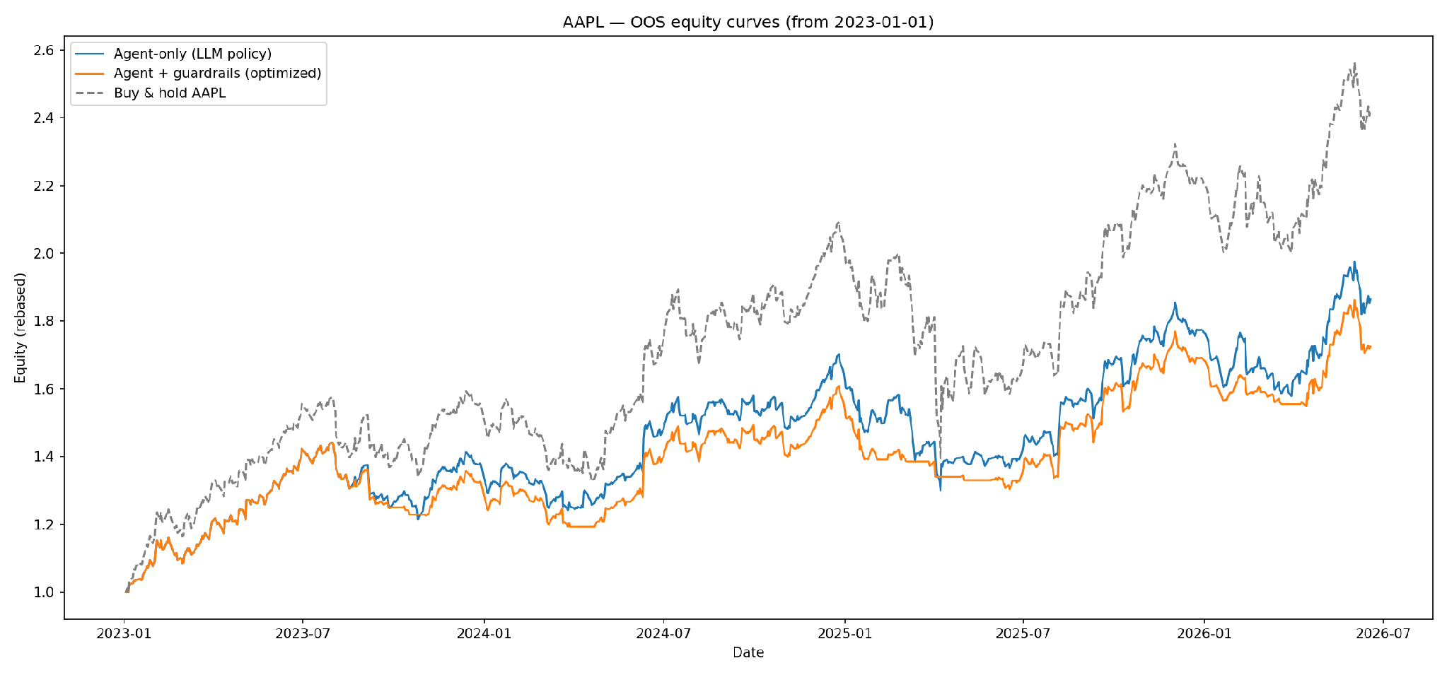
Figure: AAPL OOS equity curves (January 2023 – present), all rebased to 1.0.

Reading the equity curves

Three observations stand out from the chart. First, all three curves rise through 2023–2024, confirming the strategy participates in AAPL's uptrend. Second, the Agent + Guardrails curve consistently stays close to the Agent-only line during rallies but detaches downward more slowly during corrections, that divergence is the guardrail doing its job: trimming exposure before losses compound. Third, Buy & Hold finishes highest because AAPL's 2023–2026 uptrend was unusually strong with shallow corrections; in a choppier or bear market, the lower volatility and smaller drawdown of the guardrailed strategy would translate into a clear risk-adjusted advantage (Calmar ratio: 0.91 vs. 0.88 for Buy & Hold).

Step 10: How to Improve the Strategy

The strategy we have just built is a working foundation. As previously mentioned, we’re here not to provide you with the best strategy, but to give you insights, tips and their reasons so you can think of improving your strategy based on them or even improve ours for further research.

Signal Quality

Multi-horizon momentum. Add 5-day and 63-day cumulative returns alongside the current 20-day trend score. The three horizons together give the LLM context about whether the stock is in an early, mid, or late-stage trend.

Earnings blackout. Force the position to FLAT_EXP in the two trading days surrounding each AAPL quarterly earnings release. Earnings dates are publicly known in advance, so this introduces no lookahead bias and prevents the strategy's worst gap-risk events.

Macro regime filter. Add a binary feature for whether the S&P 500 is above or below its 200-day moving average (you can even optimize that window). This gives the LLM a market-wide context that is especially useful during broad corrections where single-stock features lag.

Volume z-score. Add today's volume relative to its 20-day average as a state dimension. Unusually low volume often precedes a reversal; unusually high volume confirms momentum.

Position Sizing

Kelly-fraction hints. Compute a fractional Kelly size per state from the training statistics and pass it to the LLM as a sizing hint. Use 25% of full Kelly to avoid overbetting on noisy estimates, and verify it improves OOS Sharpe before keeping it.

Regime-conditional leverage cap. During VOL_HIGH states, tighten MAX_LEVERAGE to 0.6 regardless of the vol-targeting output. This prevents rebuilding a full position into a still-stressed market after a guardrail re-entry.

Continuous size output. Ask the LLM to output a continuous exposure in [0, 1] rather than three discrete levels. This produces finer-grained position modulation and smoother equity curves, at the cost of tighter output validation.

Guardrail Robustness

Relative drawdown limit. Replace the absolute DD stop with one that compares strategy equity to buy-and-hold over the same window. This prevents false exits during bull markets where an absolute drawdown is still a relative outperformance.

Noise-filtered vol stop. Require three consecutive days of elevated volatility before the stop fires, rather than reacting to a single day. This removes most spurious triggers from one- or two-day spikes that quickly revert.

Separate cooldowns. Give the vol stop and the drawdown stop their own cooldown counters (for example, 3 days and 15 days respectively). Vol spikes normalise quickly; drawdowns can persist for weeks.

Guardrail optimisation frequency. Test annual, semi-annual, and quarterly reoptimisation cadences to find the right balance between adaptability and overfitting. For slow-moving regimes, annual reoptimisation may be more robust than the current quarterly default.

LLM Prompting

Comparative ranking prompt. Ask the LLM to rank all states by risk/reward and assign exposure by rank tier (top 50% get full, bottom 25% get FLAT). This prevents the degenerate case where the model assigns LONG to every state because each looks acceptable in isolation.

Regime classification first. Ask the LLM to classify the overall regime (BULL, CHOP, or STRESS) before setting per-state exposure. This anchors all decisions to a coherent macro view and produces a loggable regime label you can plot over the OOS period.

Multi-model comparison. Run the same prompt through a second model (GPT-4o or Claude) and compare OOS policies. Systematic agreement between models can be a stronger evidence of signal quality than results from a single model.

Evaluation

Rolling Sharpe chart. Plot the rolling one-month Sharpe over the OOS period. A single aggregate Sharpe number hides whether the edge is persistent or concentrated in one lucky window.

Vol-targeted benchmark. Add a vol-targeted buy-and-hold (always long, same vol-scaling as the strategy) to the metrics table. If the LLM strategy cannot beat this benchmark, the vol-targeting module is doing all the work.

Transaction cost sensitivity sweep. Report results at 0.5, 1.0, and 2.0 bps total cost. A strategy that only works at best-case IBKR pricing is fragile; one that holds up at 2.0 bps has a more durable edge.

Frequently Asked Questions

Q: Why use an LLM for this at all? Couldn't a simple rule do the same thing?

Yes: and we built exactly that comparison into the notebook (POLICY_MODE='rule'). Run both and check the metrics. If the rule beats the LLM, the LLM isn't adding value and you should drop it. The goal of including both is intellectual honesty: the LLM should only stay in the strategy if it demonstrably improves something. In our tests, the LLM's benefit was in smoother decision-making across borderline states: cases where the statistics are ambiguous and a rule-based threshold would flip noisily.

Q: What is the guardrail deadlock and why does it matter?

When a drawdown stop fires and position goes to zero, equity freezes. A frozen equity means the drawdown never mathematically improves. So the drawdown check fires again the next day: and the next: locking the strategy flat indefinitely. The MAX_FLAT_DAYS re-entry counter fixes this by forcing a partial re-entry after one trading month regardless of the drawdown level.

Q: Can I use this on other stocks?

Yes, with two adjustments. First, change SYMBOL and re-download data. Second, the LLM policy cache is keyed by symbol, so you will need fresh API calls for the new ticker. The architecture works for any liquid single stock or ETF with a long price history. For assets with less history than AAPL, reduce TRAIN_YEARS to 2, or the state statistics will be too sparse.

Q: How much does the DeepSeek API cost to run this?

The walk-forward loop makes approximately 40 API calls (one per OOS month) with max_tokens=2000 each. DeepSeek-chat is among the most cost-efficient frontier models: the full OOS run costs under $0.10 at current pricing. The policy cache means re-runs are free once the cache is warm.

Q: What is the next step to improve performance?

The single highest-impact improvement is better state features. The current three-feature state space (trend, vol, z-score) is coarse. Try using ta-lib technical indicators to improve the signal quality meaningfully.

Conclusion

What we built here is a framework for thinking about LLM-assisted risk management: not a magic alpha-generating machine. The honest summary is this: the LLM earns its place in this strategy not by predicting the market, but by making nuanced distinctions between market states that a simple rule would handle with a blunt threshold.

The architecture has three layers, and each does something distinct. Feature engineering and state bucketing translate raw price action into something a language model can reason about. The LLM prompt, framed as a risk manager rather than a forecaster, sets a monthly exposure policy across those states. And the hard guardrails: with their re-entry mechanism: ensure that no single bad patch of markets can permanently sideline the strategy.

The results show a strategy that participates meaningfully in AAPL's upside while cutting maximum drawdown by 45% (from -33% to -18%) versus buy-and-hold. That is a legitimate and useful property for a real portfolio. Is it the final word? Absolutely not. The state features are coarse, the LLM prompt is version 1, and the guardrail thresholds could be smarter. But the framework is sound, the walk-forward methodology is honest, and every design decision is traceable.

The best way to learn from this is to run it, break it, and rebuild it. Change the prompt. Add a momentum feature. Swap AAPL for SPY. See what happens. The notebook is built to be modified: everything flows from the settings cell at the top.

References

[Chan, 2024] E. P. Chan, “Machine Learning in Trading,” YouTube, 2024. Available: https://www.youtube.com/watch?v=VzF-tvz3DAk&t=411s

Note:

The strategy idea originated from the author

The blog content was created with the assistance of an AI large language model and

The blog content was curated/edited by the author.

Disclaimer: This blog is for educational and illustrative purposes only. Trading in financial markets involves substantial risk of loss. The code and concepts discussed here are not financial advice. Always exercise caution and thoroughly understand any automated trading system before deploying it in a live environment.

Summer Sale july 2026