
Cross Validation (CV) is not a novel topic, but from my experience as both a data scientist and front desk practitioner, it is a statistical tool often underappreciated and misused. I believe that innumerous bad trading ideas could have been discarded had they been handled with due statistical care. So this blog is both a cautionary tale and a quick reference to modern CV methods in finance.
We will cover the following topics:
- Embargoing
- Purging
- Backtesting through Cross Validation
- Combinatorial Purged Cross Validation
- Example of Combinatorial Purged Cross Validation in Python
Cross validation in machine learning has been covered previously, and I'd like to focus here on the topic of cross-validation as a backtesting tool. I will mention some of the pitfalls of cross validation (CV) in finance as well, specially in what concerns data leaking and data peeking.
To recap, CV is a resampling tool aimed at assigning measures of accuracy (e.g.: bias, variance, confidence intervals, prediction error, etc.) to sample estimates (e.g.: model performance, Sharpe values etc). CV is an old idea in statistics whose time seems to have come back again with the advent of modern computers and machine learning.
In finance, CV becomes especially important in handling the high noise-to-signal effects, and in mitigating spurious results resulting from the overfitting of strategies. I should also say that CV is not restricted to ML trading models only, and can be applied to rules-based strategies created through data mining.
Embargoing
I will be using both terms (data leaking and data peaking) interchangeably in the context of CV. This refers to situations where information deliberately or not leaks across folds. This is important when your model or strategy contains indicators that require historic data with large lookbacks.
Let's use a concrete example for illustration. For sake of concreteness, assume that
- Your model or strategy depends on an indicator such as realised volatility with a lookback of 63 days (or 3 business months)
- Your folds are ordered chronologically, in 1 year blocks
- Your current test or out-of-sample fold is year 4
Schematically, the folds would look like this: |--1--||--2--||--3--|(|--4--|)|--5--|
Between years 4 and 5, volatility computed in the early days of year (5) would require information that's only available in the OOS fold. (There's no issue between folds 3 and 4 since the information required in fold 4 is already available.)
One common approach to dealing with this unintended data leak is to use what De Prado calls purging and embargoing. In technical terms, this involves removing some of the data points near the boundaries of affected folds, but there's a subtle difference between the two processes.
There's more to it than I'm mentioning here since in De Prado's terminology, to each labelled data point there are two times attached to it: a trade time and an event time. The specific type of data removal I'm suggesting in the example above is an example of embargoing. (It happens before purging.) In our specific example, I'd remove the first 63 or so days from fold (5).
Moral: Be aware of the temporal dependencies of your features.
Purging
Before we discuss purging, we need to talk about event times in finance. In essence, this means that any labelled data point in a financial time series has a trade time and an event time. The event time usually indicates when in the future the mark-to-market value of an asset reached a certain level such as a stop loss or a take profit price. In practice, this means that labels become path-dependent, and care needs to be taken so that when computing labels we don't peek into the out-of-sample fold.
For a concrete example, say we are trying to build an ML model to predict whether IBM prices would move up or down in the next 5 business days by at least 50 basis points (bps) based on various data sources. The size of these movements are estimated based on recent levels of realised volatility for IBM shares. A common labelling scheme would be: +1 if the share price moves more than 50 bps, 0 if the share price moves by less than 50 bps in absolute value, and -1 if the share price moves down by more than 50 bps.
Next, let's assume that our typical trading horizon is 1 week. You would enter a position today, and liquidate it one week later. Most people in practice however would have a stop loss or take profit level for a trade so that they can exit a trade earlier if either of those levels are reached. The point is that to mark-to-market your trade, you'd need to observe the price path during the next 5 days, or for the next 5 ticks (you could exit before).
In the labelling process, we have to take care to remove data for which the event times overlap with the trade times in the test fold. This process is called purging.
In practice, one first embargoes the data set, and then purges it. One can implement embargoing by increasing the event time of the test fold preceding a training fold. (See De Prado for more details.)
Moral: Be aware of the price paths between trades and events (e.g. end of the trading horizon, stop loss, take profit etc.)
For more in-depth information on this topic of label building in finance, I recommend the Financial Data Science & Feature Engineering introductory video from Quantra.
Backtesting through Cross Validation
Once you develop a strategy, rule-based or ML-based, it's time to backtest it. The first time around you obtain a Sharpe ratio (SR) of 0.5 and unhappy with your results you decide to tweak your strategy. Perhaps, you tell yourself you should use a different threshold level for that first indicator and see what happens, or a higher value for that other ML hyperparameter.
The course emphasizes the importance of backtesting through cross-validation to ensure robustness and avoid overfitting. By systematically adjusting your strategy and assessing its performance, you can optimize the approach and improve your results over time.
Maybe I should also try different enter/exit times throughout the day. Eventually, after multiple iterations of tweaking this or that parameter, you end up with a "flawless" combination of parameters and a strategy with a Sharpe ratio of 2.0.
Incredible! Now you are ready to trade.
However, in live trading your performance took a different turn: you essentially tanked and lost money. What went wrong?
I'm using this made up example to illustrate the concept of an overfit strategy, and to illustrate where CV could come in handy to assist you in assessing the statistical significance of your results.
You could use the same process where you can split your data into folds, and perhaps repeat the same process above of calibrating the parameters in the IS folds, and backtesting the strategy in the OOS fold.
Is your choice of parameters robust in the IS folds?
Is your performance robust on the OOS folds?
If so, you have more statistical evidence of the soundness of your strategy. (Otherwise, you're shooting in the dark, and as a quant investor we should not leave room for second-guessing.)
This exercise also enables you to discard some trading parameters that are too unreliable to be used in live trading since their prominence in the backtest was probably due to overfitting.
Most of us in the machine trading space are familiar with CV for ML strategies, but as illustrated above, it can be used for rule-based strategies too. One positive outcome of the CV inspired backtest is that you can obtain a true estimation of performance across the entire market history you're investigating -- whether that's a 5 years window (for daily traders), or 1 week worth of data for high-frequency traders.
Moral: Backtesting is not a research tool. Avoid selection bias on multiple backtests because you'll be falsely monetising on random historic patterns. (Quite a lot of research in finance is still driven by backtests.)
De Prado for instance, in [AFML] has various suggestions on how to prevent backtest overfitting:
1. Develop models for entire asset classes or investment universes, rather than for specific securities
2. Apply ensemble techniques as means to both prevent overfitting and reduce the variance of the forecasting error (see Quantra course on trees for trading)
3. Do not backtest until your research is complete
4. Stress test your strategies with various "what if" scenarios
5. If the backtest fails to identify a profitable strategy, start from scratch.
This demands a lot more discipline and due skill, but it can potentially spare you from a lot of frustration and wasted money.
Combinatorial Purged Cross Validation
One of the main drawbacks of the standard CV approach in finance is that CV tests only a single path. In the absence of a market simulator, one alternative approach is to use some combinatorial tricks to generate multiple backtest paths.

For this part of the blog, I will provide some Python code illustrating how to build 5 backtest paths out of 1 historical path using the so-called combinatorial purged cross-validation. (See the diagram above.) I'm going to use a specific example here.
Example of Combinatorial Purged Cross-Validation in Python
We will first download the required libraries

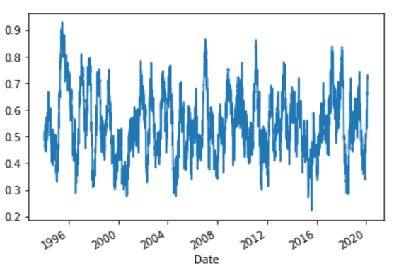
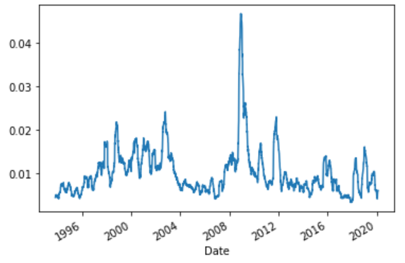
We will print the number of days in the dataset and also plot the volume graph.

Further, we will install hurst package.
Let us plot the percentage change now

The output is as follows:
1 4710
0 2101
Name: signal_mh, dtype: int64


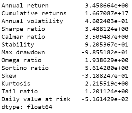
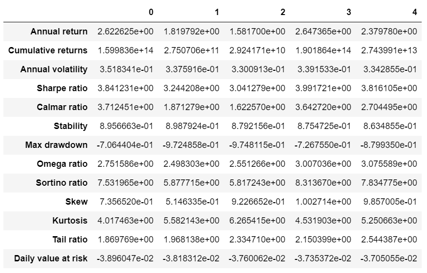
The Sharpe Ratio for this baseline strategy over the entire history of the data is about 3.49, which seems exceptional. However, notice how volatile the strategy has been in the last 3 years. Other metrics to bear in mind are max drawdown: here the worst drawdown has been 98%, which would have wiped out your wealth nearly entirely.
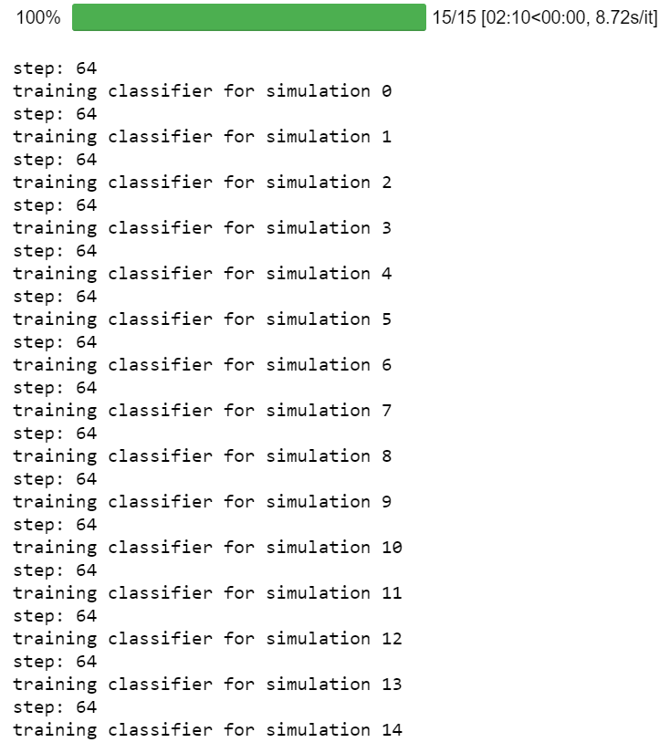
n_sim: 15
n_paths: 5

0.018698578908002993


(6685, 16)
1.0 3468
0.0 3196
(6664, 6664)
6403
n_sim: 15
n_paths: 5
3.58690887256234
0.4172048765982637

-0.8520855548962698
0.12966661714422806

Try modifying the above code and adapt it for other possible quantamental situations. The true challenge is estimating the real gain of a quantamental approach to baseline strategy.
Conclusion
The topic of cross-validation for backtesting is an extensive one, and I recommend readers to read more about the subject on both De Prado's AFML or on Campbell et al.
A Backtesting Protocol in the Era of Machine Learning [PDF Link]
However the topic is well-documented, and there are open source libraries in Python that a hobbyst or professional trader could leverage in their research pipelines such as timeseriescv [Github Link]
The code as well as the data file used in this available in the download section below. Do feel free to post your feedback or any queries in the comments.
Download Data File
- SPY Data
- Cross validation code
The views, opinions, and information provided within this guest post are those of the author alone and do not represent those of QuantInsti®. The accuracy, completeness, and validity of any statements made or the links shared within this article are not guaranteed. We accept no liability for any errors, omissions or representations. Any liability with regards to infringement of intellectual property rights remains with them.
