Machine Learning Strategy using Blueshift Visual Programming

By Gaurav Singh

Algo trading is all about how well you research, backtest, analyze and then live trade your strategy. Blueshift® is a platform where you can construct, analyse and trade your systematic investment strategies. On Blueshift, you can backtest your strategies on historical data. After satisfactory backtesting results, you can paper trade or live trade by connecting your broker with Blueshift. What's great about Blueshift is that it is a free-to-use platform!

You can see how the completed machine learning strategy will look like on Blueshift. Just click on the button below! A new window will open, with the pre-built strategy as discussed in this blog.

View the Strategy on Blueshift!

In this article, you will learn to construct a machine learning strategy. You can easily make this strategy using Blueshift’s cool new addition, the Visual Programming interface. The strategy will be built without writing a single line of computer code! Also, no special software installation is required in your system. Everything will be done on the Blueshift platform!

This article covers:

• What is Blueshift’s Visual Programming?
• Machine Learning Pipeline in Blueshift’s Visual Programming
• Building a Machine Learning Strategy
• Backtesting and Live Trading the Strategy
• Future Enhancements to the Strategy

What is Blueshift’s Visual Programming?

There are a lot of people who have a lot of trading experience, but they are not adept in computer programming. This adds a significant entry barrier for a person to take part in algorithmic trading. Blueshift has recently added a feature called visual programming. This feature enables you to create strategies without any knowledge of coding. That’s right, you can create the strategy by only drag and drop the strategy building blocks!

You can check out the 7-part youtube series on Blueshift’s Visual Programming. The series explains the user interface and different features of the platform. It also constructs a simple crossover strategy.

Machine Learning Pipeline in Blueshift’s Visual Programming

Visual Programming is not merely an easy to use interface for defining a set of simple trading rules. Visual Programming is an almost complete programming language capable of handling any logic.

This means you can also build complex strategies such as machine learning models. You can use Blueshift to backtest or live trade a machine learning strategy as easily as you can backtest a simple crossover strategy. If you are not familiar with machine learning, you can do the free course Introduction to Machine Learning for Trading on Quantra!

Underneath the easy to use interface, lies an intelligent software engine which validates and converts the visual blocks into python code. The machine learning pipeline in Blueshift’s visual programming follows the sklearn pipeline flow.

Don’t worry if you are not familiar with the pipeline terminology! A pipeline is simply a set of transformers and estimators applied to a data set. In other words, a sequence of mathematical operations is applied to transform the data appropriately. Then, the estimator essentially tries to find patterns in the data. This pattern finding is also called “model fitting”. The measure of how well the model is “fit” over new data is called “score”. The “score” gives insight into how accurately the model can predict any unseen data.

The last estimator in the machine learning pipeline only needs to implement the “fit” function and get the results. The score calls the underlying “score” function of the estimator.

The following diagram gives an idea of how the machine learning model is built and used, along with the relevant Blueshift visual programming blocks alongside. The model is built by adding the features, target and estimators. Ideally, the features should be uncorrelated amongst themselves and be weakly predictive. The target is the dataset which is or should be the machine learning output.

The estimator is chosen based on the problem statement at hand. For example, if the final output is the predicted price, then the regression estimator is used. But if the final output is a classification (to maintain a long position or to maintain no position) then the classifier estimator is used.

Note: the target can be both for regression (no levels required) and classification (requires levels).

The model is then compiled and fit using the “estimate” block. Then the model predictions are computed using the “predict” block. And finally, the model is scored on the unknown data using the “score” block.

Building a Machine Learning Strategy

In this article, you will learn how to construct a long-only machine learning model using the Random Forest Classification estimator. That means, the strategy will only take long positions and the underlying machine learning estimator is the random forest classifier.

The key backtesting results which you can expect from the strategy (backtest starting from January 2015 till November 2020) you build here are as follows:

Note: The backtesting results will vary slightly each time you run the model. This difference is due to the inherent randomness in the random forest algorithm used by the model to fit the data.

Now, let’s create this strategy using Blueshift’s Visual Programming. If you are not familiar with the user interface, you can refer to the Interface Overview video.

The strategy is constructed by following these steps:

Strategy Settings

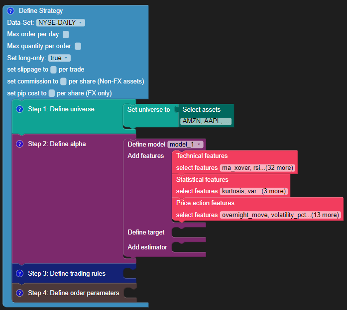
The initial strategy block looks as follows:

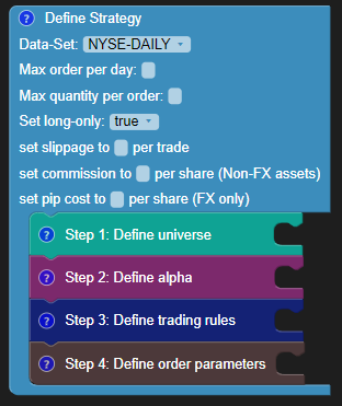
Make sure to select the dataset as NYSE-DAILY as you will be designing the strategy based on daily NYSE data. As you are making a long-only strategy, set the long-only option to “True”. To know more about each parameter, you can refer to the Strategy Settings And Trade Universe video.

Define the Universe

Connect the “set universe to” and the “select assets” blocks to the “Define Universe” step. For this sample strategy, you can choose these stocks: AMZN, AAPL, WMT, MU, BAC, KO, BA, AXP.

Define the Alpha (Machine Learning Model)

The alpha of your strategy will be the prediction output from the machine learning model. So you need to define the machine learning model as your strategy alpha. To refresh your memory about alpha and variables, you can refer to the Variables And Alpha Functions video.

Create a model using the "Use model" in the Machine Learning menu on the left. You can name the model as “model_1”.

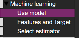
Connect the “model_1” block to the "Define alpha" step.

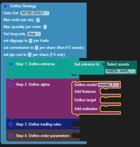
To define the model, you need to specify these three things:

1. Features
2. Target
3. Estimator

Features

The features available in Blueshift Visual Programming are as follows:

1. Technical: crossovers, MFI, RSI, Fibonacci and more
2. Statistical: kurtosis, var, mean, median and more
3. Price action trading features: doji, engulfing, gap-up/down, and more

You can use any combination of these features and analyse the performance. It is very easy to add features to your model. Just connect the relevant block to the “Add Features” and click on select features.

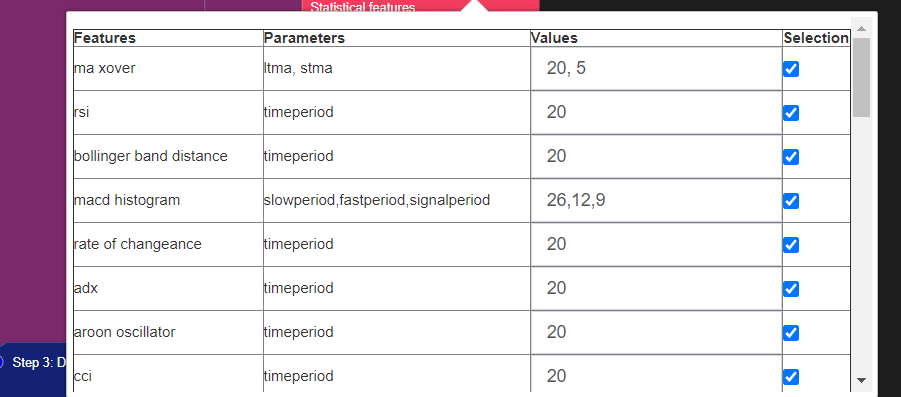
A menu shows which features are available and which ones are currently selected.

The features used in this sample strategy can be seen by loading the pre-built strategy at the end of this section.

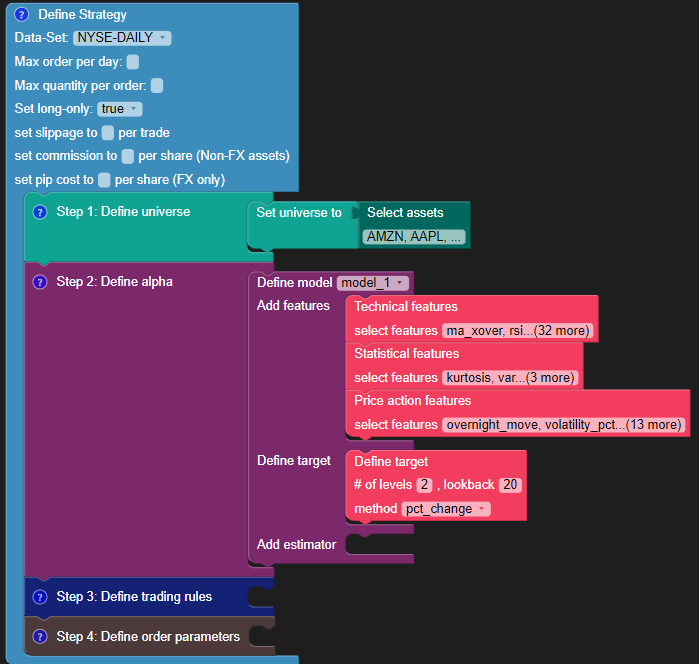
Target

The target maps price returns performance (based on close-to-close price) automatically to the estimator target (classification or regression output). The inputs required for defining a target are:

1. The number of levels of encoding: In the sample classification strategy, you can either “maintain a long position” or “maintain no position”. Thus the level of encoding will be two. If the estimator is of regression type, then the number of levels will be zero.
2. Lookback period: The lookback period for return calculation.
3. Method of measuring return performance: To use percentage change or difference when calculating the returns. For the sample strategy, choose the “pct_change” option.

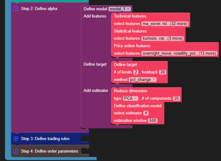
Estimator

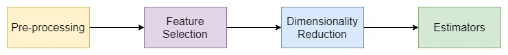
In addition to pre-processing and feature selection, you can use the machine learning pipeline in Blueshift Visual Programming for dimensionality reduction. In the end, you add an estimator to obtain the model output.

The available options are:

1. Feature Selection: to select the k-best features
2. Dimensionality Reduction:
   a) PCA
   b) Linear kernel PCA
   c) rbf kernel PCA
3. Estimator and the rolling estimation window:
   a) Classification: Logit, ridge, random forest, xgboost, etc
   b) Regression: OLS, lasso, ridge, random forest, etc

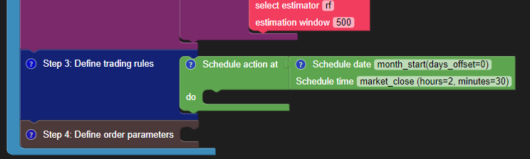
For your strategy, select the PCA dimensionality reduction to 25 components. Select the classification estimator block and the estimator as “rf” (random forest) with a rolling estimation window of 500 periods (approximately 2 years on daily frequency data).

Define the Trading Rules and Trade Schedule

You will now define the trading rules and schedule your strategy. If you are not familiar with the trading rule blocks, you can refer to the Trading Rules And Actions and Scheduling and Order Parameters tutorial videos.

The sample strategy trades on the first day of each month, 2.5 hours before the market closes.

Add the scheduling block accordingly.

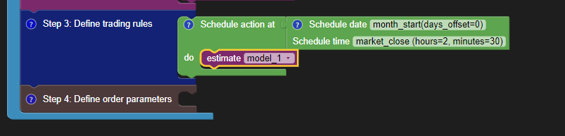
Then, you need to compile and fit the model before you can use its predictions. You compile and fit the model by using the “estimate” block.

Now you are ready to utilise the model. But, do you want to use the model all the time?

No! You don’t want to use the model when the model accuracy is worse than a random prediction. So you add a logical “if condition”, which states that we will use the model only if the model score is better than 0.5 (50% mean accuracy).

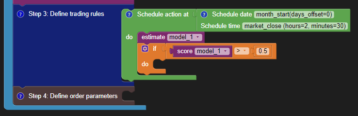
The “score” block calls the underlying sklearn score function of the estimator. As you are using the random forest classifier, it will give you the mean accuracy on the given test data and labels (Source).

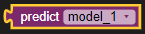
Now, you will use the “predict” block to know whether the model predicts it as class 0 (maintain no position), or class 1 (maintain long position).

You can make a long-entry for classification output 1. And long-exit for classification output 0. You have learnt these in the Trading Rules And Actions video.

The order type is set as “portfolio fraction” of 0.1 with “target” type method. This means that you will take positions in the assets such that 10% of the available portfolio wealth is allotted to the long position. Similarly, if the classification output is 0, you exit the long position.

Your strategy is now complete! You can click this button to launch Blueshift Visual Programming with this strategy pre-built!

Launch the Pre-built Strategy on Blueshift

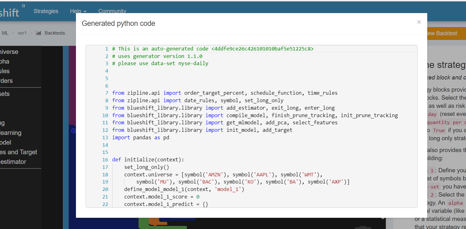
You can also view the automatically generated code by clicking the “View Code” button in the lower right section of the screen.

The generated code can be seen in a new popup window. All the blocks from the visual programming interface are converted to python code which will be then run by the Blueshift platform.

Backtesting and Live Trading the Strategy

You can obtain the detailed backtest for the machine learning strategy by clicking on the “New Backtest” button. Choose the dataset as NYSE-DAILY and backtest the strategy from January 2015 to November 2020.

The key performance metrics are as follows:

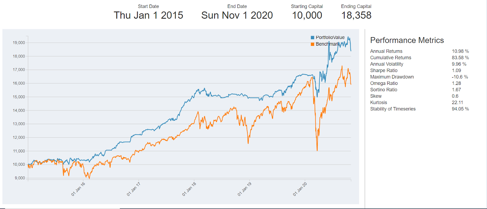
It is interesting to note that the benchmark returns went down significantly in early 2020 due to the COVID-19 pandemic. But, the portfolio returns remarkably outperformed the benchmark in the early months of 2020.

In general, the strategy avoided heavy drawdowns when the benchmark returns dipped suddenly. A Sharpe ratio of 1.09 over the course of almost 5 years is also considered good.

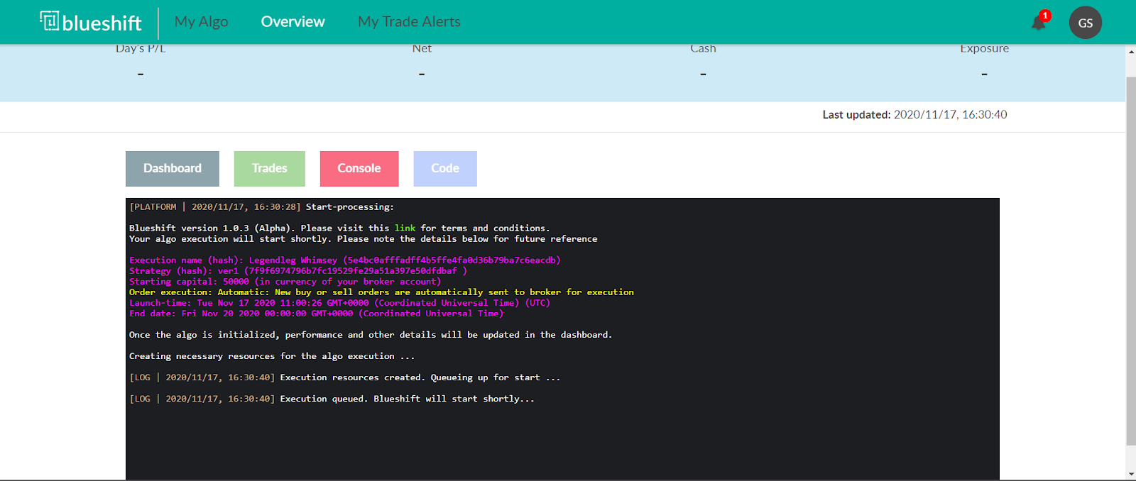
After satisfactory backtesting results, you can paper trade and then live trade your model! Just click on the “Go Live” button.

Follow the steps on screen to trade your strategy live! You can refer to the Backtesting And Live Trading video to see each step in detail.

Once you connect your broker and add the strategy settings, the strategy is set to trade on the live price date. You can analyse the trade logs, strategy metrics and the console output in the live trading overview.

Future Enhancements to the Strategy

The strategy you learnt here implements a random forest classifier based on several features. You can play around with a different combination of input features to see if you improve the performance. As shown earlier, the feature selection is possible from the easy to use graphical interface. You just need to connect the relevant block to the “Add Features” and select from the menu.

You can also change the strategy hyperparameters like lookback window and number of estimators. The machine learning model will perform differently for different assets in your trade universe. You can change the tradable assets and analyse the performance.

You can add complex risk management trading rules with different stop loss and take profit criteria. Feel free to tweak this strategy to suit your needs!

You can refer to the visual programming tutorial series if you need to recall how to use the interface or any of the blocks.

If you need any help or support, reach out to us via the Quantra Community Forum, or write to us at blueshift-support@quantinsti.com.

Disclaimer: All investments and trading in the stock market involve risk. Any decisions to place trades in the financial markets, including trading in stock or options or other financial instruments is a personal decision that should only be made after thorough research, including a personal risk and financial assessment and the engagement of professional assistance to the extent you believe necessary. The trading strategies or related information mentioned in this article is for informational purposes only.