Decision Tree For Trading Using Python

By Mario Pisa Peña

Decision Trees, are a Machine Supervised Learning method used in Classification and Regression problems, also known as CART.

Remember that a Classification problem tries to classify unknown elements into a class or category; the output always are categorical variables (i.e. yes/no, up/down, red/blue/yellow, etc.)

A Regression problem tries to forecast a number such as the return for the next day. It must not be confused with linear regression which is used to study the relationship between variables. Although the classification and regression problems have different objectives, the trees have the same structure:

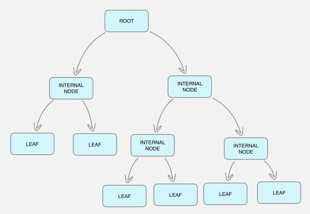
• The Root node, is at the top and has no incoming pathways.
• Internal nodes or test nodes are at the middle and can be at different levels or sub-spaces, and have incoming and outgoing pathways.
• Leaf nodes or decision nodes are at the bottom, have incoming pathways but no outgoing pathways and here we can find the expected outputs.

Thanks to Python’s Sklearn library, the tree is automatically created for us taking as a starting point the predictor variables that we hypothetically think are responsible for the output we are looking for.

In this introduction post to decision trees, we will create a classification decision tree in Python to make forecasts about whether the financial instrument we are going to analyze will go up or down the next day.

We will also make a decision tree to forecasts about the concrete return of the index the next day.

Preparing The Environment

Be sure you have available the following software pieces in order to follow the examples:

• Python 3.6
• Pandas library for data structure.
• Numpy library with scientific mathematical functions.
• Quandl library to retrieve market data.
• Ta-lib library to calculate technical indicators.
• Sklearn ML library to build the trees and perform analysis. (among many others things)
• Graphviz library to plot the tree.

Building a Decision Tree

Building a classification decision tree or a regression decision tree is very similar in the way we organize the input data and predictor variables, then, by calling the corresponding functions, the classification decision tree or regression decision tree will be automatically created for us according to some criteria we must specify.

The main steps to build a decision tree are:

1. Retrieve market data for a financial instrument.
2. Introduce the Predictor variables (i.e. Technical indicators, Sentiment indicators, Breadth indicators, etc.)
3. Setup the Target variable or the desired output.
4. Split data between training and test data.
5. Generate the decision tree training the model.
6. Testing and analyzing the model.

If we look at the first four steps, they are common operations for data processing. If you are a newcomer to decision trees the predictor and target variables may sound exotic to you. However, they are nothing more than additional columns in the data frame that contain some type of indicator. These indicators or predictors are used to predict the target variable that is the financial instrument will go up or down for the classification model, or the future price level for the regression model. Likewise, splitting data is a mandatory task in any backtesting process (ML or not), the idea is to have one set of data to train the model and another set of data, which have not been used in training, to test the model.

Steps 5 and 6 are related to the ML algorithms for the decision trees specifically. As we will see, the implementation in Python is quite simple. However it is fundamental to understand well the parameterization and the analysis of the results. This post is eminently practical and to go deeper into the underlying mathematics we recommend reading the references at the bottom of the post.

Getting the data

The raw material for any algorithm are data. In our case they would be the time series of financial instruments, such as indices, stocks etc. and it usually contains details like the opening price, maximum, minimum, closing price and volume. This information is recorded at a certain frequency, such as minutes, hours, days or weeks, and forms a time series.

There are multiple data sources to download the data, free and premium. The most common sources for free daily data are Quandl, Yahoo or Google or any other data source we trust.

Here, we are going to work with twenty years of daily data from the Emini S&P 500 that we will retrieve through Quandl.

import quandl
df = quandl.get("CHRIS/CME_ES2")
df.head()
df.tail()
df.shape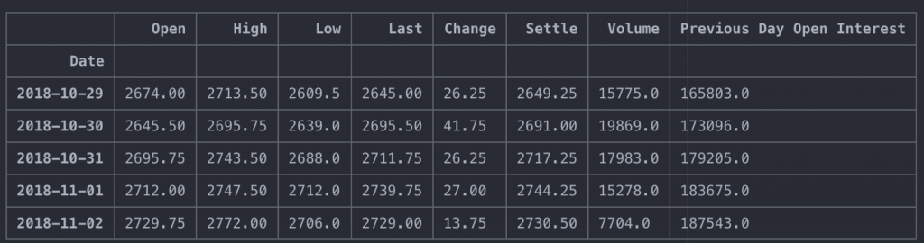

(5391, 8)

We now have just over 21 years of Emini S&P500 data available. We will use the settle price as the closing price reference.

Creating the predictors

Predictor variables are data that we think are related to market behavior. These data can be very diverse such as the technical indicators, market data, sentiment data, breadth data, fundamental data, government data, etc. that will help us to make forecasts about the future behavior of the market.

Here we will test the classical indicators for trend following and for range trading, these are:

• EMA
• ATR
• ADX
• RSI
• MACD

Therefore, the decision tree algorithm should help us select the best combination of indicators along with their parameters that maximize the expected output which is the target.

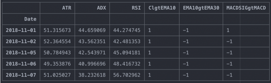
We are going to prepare the data by calculating the indicators that we will use as predictors, to do it, we will use the Ta-lib library:

import talib as ta
df['EMA10'] = ta.EMA(df['Settle'].values, timeperiod=10)
df['EMA30'] = ta.EMA(df['Settle'].values, timeperiod=30)
df['ATR'] = ta.ATR(df['High'].values, df['Low'].values, df['Settle'].values, timeperiod=14)
df['ADX'] = ta.ADX(df['High'].values, df['Low'].values, df['Settle'].values, timeperiod=14)
df['RSI'] = ta.RSI(df['Settle'].values, timeperiod=14)
macd, macdsignal, macdhist = ta.MACD(df['Settle'].values, fastperiod=12, slowperiod=26, signalperiod=9)
df['MACD'] = macd
df['MACDsignal'] = macdsignal
df.tail()

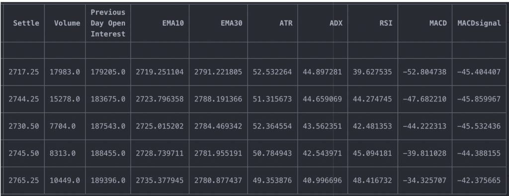
We have already calculated the indicators, but it is necessary to emphasize that we have calculated them with the standard parameters and these can, and must be optimized since the decision tree works with the pre calculated indicators.

On the other hand, EMAs and MACDs do not serve as they are, since the signal comes from the price in relation to averages, or from one average in relation to the other. Let’s calculate the columns that will serve as predictors for the averages and the MACD.

import numpy as np
df['ClgtEMA10'] = np.where(df['Settle'] > df['EMA10'], 1, -1)
df['EMA10gtEMA30'] = np.where(df['EMA10'] > df['EMA30'], 1, -1)
df['MACDSIGgtMACD'] = np.where(df['MACDsignal'] > df['MACD'], 1, -1)
df.tail()

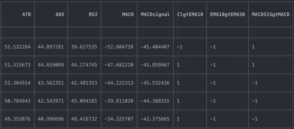
What we have now are possible trading rules that we will introduce in the decision tree to help us identify the best combination of these indicators to maximize the result.

• EMA, we are interested in when the price is above average and when the fastest average is above the slowest average.
• ATR(14), we’re interested in the threshold that will trigger the signal.
• ADX(14), we’re interested in the threshold that will trigger the signal.
• RSI(14), we’re interested in the threshold that will trigger the signal.
• MACD, we are interested in when the MACD signal is above MACD.

In this example, the predictor variables for the classification decision tree and the regression decision tree will be the same, although the target variables are different because for the classification algorithm the output will be categorical and for the regression algorithm the output will be continuous.

Learn how to make a decision tree to predict the markets and find trading opportunities using AI techniques with our Quantra course.

Creating the target variables

As we have already said, the classification and regression decision trees have different objectives. While the classification decision tree tries to characterize the future by offering a categorical variable, i.e. the market goes up or down, the regression decision tree tries to forecast the future value, i.e. the future market price.

We are going to create here the target variables for the two types of problems, although each one will use its own target.

df['Return'] = df['Settle'].pct_change(1).shift(-1)
df['target_cls'] = np.where(df.Return > 0, 1, 0)
df['target_rgs'] = df['Return']
df.tail()

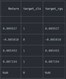
The target variable for the regression algorithm (target_rgs) uses the lagged return, this is so, because we want the algorithm to learn what happened the next day, based on the information available at the present time.

The target variable for the classification algorithm (target_cls) also uses the lagged return, but because the output is categorical, we must transform it. If the return was positive, we assign 1 and if it was negative, we assign 0.

Obtaining the data set for decision trees

We have all the data ready! We have downloaded the market data, applied some technical indicators as predictor variables and defined the target variable for each type of problem, a categorical variable for the classification decision tree and a continuous variable for the regression decision tree.

We are going to do a small operation to sanitize the data and prepare the data set that each algorithm will use. We must clean the data dropping the NA data, this step is crucial to compute cleanly the trees.

Next, we are going to create the data set of the predictor variables, that is to say, the indicators that we have calculated, this data set is common to the two decision trees that we are going to create, a classification decision tree and a regression decision tree.

predictors_list = ['ATR', 'ADX','RSI', 'ClgtEMA10', 'EMA10gtEMA30', 'MACDSIGgtMACD']
X = df[predictors_list]
X.tail()

We then select the target dataset for the classification decision tree:

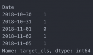
y_cls = df.target_cls
y_cls.tail()

Finally, we select the target dataset for the regression decision tree:

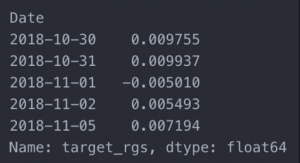
y_rgs = df.target_rgs
y_rgs.tail()

Splitting the data into training and testing data sets

The last step to finish with the preparation of the data sets is to split them into train and test data sets. This is necessary to fit the model with a set of data, usually 70% or 80% and the remainder, to test the goodness of the model. If we do not do so, we would run the risk of over-fitting the model. We want to test the model with unknown data, once the model has been fitted in order to evaluate the model accuracy.

We’re going to create the train data set with the 70% of the data from predictor and target variables data sets and the remainder 30% to test the model.

For classification decision trees, we’re going to use the traintestsplit function from sklearn modelselection library to split the dataset. Since the output is categorical, it is important that the training and test datasets are proportional traintest_split function has as input the predictor and target datasets and some input parameters:

• test_size: the size of the test data set, in this case, 30% of the data for the tests and, therefore, 70% for the training.
• random_state: Since the sampling is random, this parameter allows us to reproduce the same randomness in each execution.
• stratify: To ensure that the training and test sample data are proportional, we set the parameter to yes. This means that, for example, if there are more days with positive than negative return, the training and test samples will keep the same proportion.

from sklearn.model_selection import train_test_split
y=y_cls
X_cls_train, X_cls_test, y_cls_train, y_cls_test = train_test_split(X, y, test_size=0.3, random_state=432, stratify=y)

print (X_cls_train.shape, y_cls_train.shape)
print (X_cls_test.shape, y_cls_test.shape)

Here we have:

• Train predictor variables dataset: X_cls_train
• Train target variables dataset: y_cls_train
• Test predictor variables dataset: X_cls_test
• Test target variables dataset: y_cls_test

For regression decision trees we simply split the data at the specified rate, since the output is continuous, we don’t worry about the proportionality of the output in training and test datasets.

train_length = int(len(df)*0.70)
X_rgs_train = X[:train_length]
X_rgs_test = X[train_length:]
y_rgs_train = y_rgs[:train_length]
y_rgs_test = y_rgs[train_length:]

print (X_rgs_train.shape, y_rgs_train.shape)
print (X_rgs_test.shape, y_rgs_test.shape)

Again, here we have:

• Train predictor variables dataset: X_rgs_train
• Train target variables dataset: y_rgs_train
• Test predictor variables dataset: X_rgs_test
• Test target variables dataset: y_rgs_test

So far we’ve done:

• Download the market data.
• Calculate the indicators that we will use as predictor variables.
• Define the target variables.
• Split the data into training set and test set.

With slight variations in obtaining the target variables and the procedure of splitting the data sets, the steps taken have been the same so far.

Decision Trees for Classification

Now let’s create the classification decision tree using the DecisionTreeClassifier function from the sklearn.tree library.

Although the DecisionTreeClassifier function has many parameters that I invite you to know and experiment with (help(DecisionTreeClassifier)), here we will see the basics to create the classification decision tree.

Basically refer to the parameters with which the algorithm must build the tree, because it follows a recursive approach to build the tree, we must set some limits to create it.

• criterion: For the classification decision trees we can choose Gini or Entropy and Information Gain, these criteria refer to the loss function to evaluate the performance of a learning machine algorithm and are the most used for the classification algorithms, although it is beyond the scope of this post, basically serves us to adjust the accuracy of the model, also the algorithm to build the tree, stops evaluating the branches in which no improvement is obtained according to the loss function.
• max_depth: Maximum number of levels the tree will have.
• min_samples_leaf: This parameter is optimizable and indicates the minimum number of samples that we want to have in leaves.

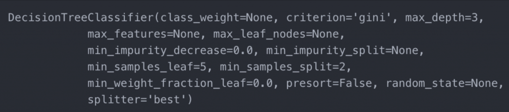
from sklearn.tree import DecisionTreeClassifier
clf = DecisionTreeClassifier(criterion='gini', max_depth=3, min_samples_leaf=6)
clf

Now we are going to train the model with the training datasets, we fit the model and the algorithm would already be fully trained.

clf = clf.fit(X_cls_train, y_cls_train)
clf

Now we need to make forecasts with the model on unknown data, for this we will use 30% of the data that we had left reserved for testing and, finally, evaluate the performance of the model. But first, let’s take a graphical look at the classification decision tree that the ML algorithm has automatically created for us.

Visualize Decision Trees for Classification

We have at our disposal a very powerful tool that will help us to analyze graphically the tree that the ML algorithm has created automatically. The graph showed the most significant nodes that maximize the output and will help us determine, if applicable, some useful trading rules.

The graphviz library allows us to graph the tree that the DecisionTreeClassifier function has automatically created with the training data.

from sklearn import tree
import graphviz
dot_data = tree.export_graphviz(clf, out_file=None,filled=True,feature_names=predictors_list)
graphviz.Source(dot_data)

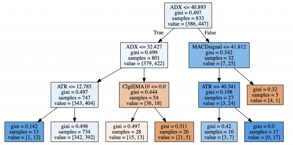
Note that the image only shows the most significant nodes. In this graph we can see all the relevant information in each node:

• the predictor variable used to split the data set.
• the value of Gini impurity.
• the number of data points available at that node and
• the number of target variable data points belonging to each class, 1 and 0.

We can observe a pair of pure nodes that allows us to deduce a possible trading rules. For example:

• On the third leaf starting from the left, when the closing price is lower than the EMA10 and the ATR is higher than 51.814 and the RSI is lower than or equal to 62.547, the marking decreases.
• On the fifth leaf starting from the left, we can deduce the following rule: When the ADX is less than or equal to 19.243 and the RSI is less than or equal to 62.952 and the RSI is greater than 62.547, the market goes up.

Make forecast

Now let’s make predictions with data sets reserved for testing, this is the part that will let us know if the algorithm is reliable with unknown data in training.

y_cls_pred = clf.predict(X_cls_test)

Performance analysis

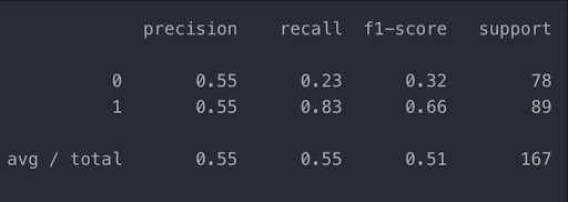
Finally, we can only evaluate the performance of the algorithm on unknown data by comparing it with the result obtained in the training process. To do this we will use the classification_report function of the sklearn.metrics library.

The report shows some parameters that will help us to evaluate the goodness of the algorithm:

• Precision: Indicate the quality of our predictions.
• Recall: Indicate the quality of our predictions.
• F1-score: Shows the harmonic mean of precision and recall.
• Support: Used as weights to compute the average values of precision, recall and F-1.

Anything above 0.5 is usually considered a good number.

from sklearn.metrics import classification_report
report = classification_report(y_cls_test, y_cls_pred)
print(report)

Decision Trees for Regression

Now let’s create the regression decision tree using the DecisionTreeRegressor function from the sklearn.tree library.

Although the DecisionTreeRegressor function has many parameters that I invite you to know and experiment with (help(DecisionTreeRegressor)), here we will see the basics to create the regression decision tree.

Basically refer to the parameters with which the algorithm must build the tree, because it follows a recursive approach to build the tree, we must set some limits to create it.

• criterion: For the classification decision trees we can choose Mean Absolute Error (MAE) or Mean Square Error (MSE), these criteria are related with the loss function to evaluate the performance of a learning machine algorithm and are the most used for the regression algorithms, although it is beyond the scope of this post, basically serves us to adjust the accuracy of the model, also the algorithm to build the tree, stops evaluating the branches in which no improvement is obtained according to the loss function. Here we left the default parameter to Mean Square Error (MSE).
• max_depth: Maximum number of levels the tree will have, here we left the default parameter to none.
• min_samples_leaf: This parameter is optimizable and indicates the minimum number of leaves that we want the tree to have.

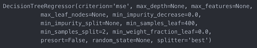
# Regression tree model
from sklearn.tree import DecisionTreeRegressor
dtr = DecisionTreeRegressor(min_samples_leaf = 200)

Now we are going to train the model with the training datasets, we adjust the model and the algorithm would already be fully trained.

dtr.fit(X_rgs_train, y_rgs_train)

Now we need to make forecasts with the model on unknown data, for this we will use 30% of the data that we had left reserved for testing and, finally, evaluate the performance of the model. But first, let’s take a graphical look at the regression decision tree that the ML algorithm has automatically created for us.

Visualize the model

To visualize the tree, we use again the graphviz library that gives us an overview of the regression decision tree for analysis.

from sklearn import tree
import graphviz
dot_data = tree.export_graphviz(dtr,
                  out_file=None,
                  filled=True,
                  feature_names=predictors_list)
graphviz.Source(dot_data)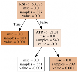

In this graph we can see all the relevant information in each node:

• the predictor variable used to split the data set.
• the value of MSE.
• the number of data points available at that node

Learn how to make a decision tree to predict the markets and find trading opportunities using AI techniques with our Quantra course.

Conclusion

It might look like we’ve found a crystal ball, but nothing could be further from the truth. Mastering these techniques requires a lot of study and an integral understanding of the mathematical techniques behind them.

Apparently, trees are easy to create and extract some rules that promise to be useful, but the truth is that to create decision trees, they need to be parametrized and these parameters can and must be optimized.

In order to continue to deepen our knowledge of decision trees and really help us to extract reliable trading rules, we will advance in the next post with the ensemble mechanisms to create a robust model combining the models created by one algorithm.

• Parallel ensemble methods or averaging methods: several models are created by one algorithm and the forecast is the average of the overall models:
  • Bagging
  • Random Subspace
  • Random Forest

• Sequential ensemble methods or boosting methods: the algorithm creates sequential models refining on each new model to reduce the bias of the previous one:
  • AdaBoosting
  • Gradient Boosting

We have learnt how to create Classification and Regression Decision Trees using Python in this blog and now we can learn advanced concepts and strategies in this course by Dr. Ernest P. Chan.

Disclaimer: All investments and trading in the stock market involve risk. Any decisions to place trades in the financial markets, including trading in stock or options or other financial instruments is a personal decision that should only be made after thorough research, including a personal risk and financial assessment and the engagement of professional assistance to the extent you believe necessary. The trading strategies or related information mentioned in this article is for informational purposes only.