This article is the final project submitted by the author as part of his coursework in the Executive Programme in Algorithmic Trading (EPAT) at QuantInsti. Do check our Projects page and have a look at what our students are building.
About the Author

Siddhant Panda holds a Bachelor of Business Administration (BBA) from SRM University and an MSc in Investment Banking and Finance from Nottingham Trent University, UK. He has six years of experience in futures and options trading, macroeconomic research and financial market analysis, and currently works as an Options Trader at Jainam Broking Pvt. Ltd. His current research interests focus on quantitative trading, particularly the integration of Deep Reinforcement Learning (DRL) into systematic trading strategies and algorithmic decision-making. He is an alumnus of EPAT Batch 69. You can connect with him on LinkedIn.
Project Abstract
Most intraday systems don’t fail because the entry signal is wrong. They fail because they trade too often, in the wrong part of the day, with costs left out of the math.
This project builds an intraday trend-following strategy on NIFTY Futures that tries to address all three. It stacks four kinds of confirmation (trend, momentum, trend strength and candle structure) using a 30-period Weighted Moving Average (WMA), a 9-period RSI, an 11-period ADX with Directional Movement (+DI/-DI), and Heikin Ashi candles. Around that sit session rules chosen by the author: no entries in the opening range, none over lunch, none after 2:15 PM, and a fixed daily loss cap.
The backtest covers June 2015 to December 2024 on 15-minute bars and includes slippage, brokerage, STT, exchange fees, GST and stamp duty. It produced 187 trades, a profit factor of 1.72 and a maximum drawdown of about 12%. Just as useful are the two checks the author ran on his own results: what the return looks like on a realistic capital base, and which exit type actually produced the profit. Both change how the headline numbers should be read, and both are covered below.
Why NIFTY Futures, and Why Multiple Filters?
NIFTY Futures are among the most liquid derivatives contracts in India, which keeps bid-ask spreads tight and makes a 15-minute strategy practical to test. Liquidity doesn’t make intraday trading easy, though. The index spends a lot of the day drifting sideways, and a trend system that trades every crossover will spend much of its time paying costs on noise.
So instead of relying on a single indicator, the author asked each candidate trade to pass several independent checks. The idea is simple: an entry should only happen when the trend, the momentum and the trend strength all agree, and when the candle itself shows conviction.
Data and Preprocessing
The strategy uses 1-minute historical NIFTY Futures data from TrueData, covering June 2015 to December 2024. Contract continuity (rolling from one expiry to the next) was handled upstream in the consolidated dataset, so the backtesting code itself contains no rollover or stitching logic. Before any indicator was calculated, the data went through these steps:
- Remove duplicate timestamps and sort strictly by date and time.
- Drop rows with missing OHLC values, non-positive prices, or a high below the low.
- Keep only NSE market hours (9:15 AM to 3:29 PM).
- Resample to 15-minute bars using right-labelled, right-closed aggregation.
def resample_ohlc(df, tf_min=15):
    x = df.set_index("DateTime").between_time("09:15:00", "15:29:00")
    agg = {"open": "first", "high": "max", "low": "min",
           "close": "last", "volume": "sum", "oi": "last"}
    out = x.resample(f"{tf_min}min", label="right", closed="right").agg(agg)
    return out.dropna(subset=["open", "high", "low", "close"]).reset_index()
The Indicator Stack
Each indicator has a specific job in the system.
| Component | Setting | Role in the strategy |
|---|---|---|
| Weighted Moving Average | 30 periods | Trend direction. Longs only above the WMA, shorts only below. |
| RSI (Wilder) | 9 periods | Momentum. Above 52 for longs, below 48 for shorts. |
| ADX | 11 periods | Trend strength. Must be between 26 and 45 and rising. |
| +DI / -DI | 11 periods | Direction of the trend, with a minimum gap of 6 points that must be widening. |
| ATR | 11 periods | Volatility filter. ATR must be at least 0.08% of price for an entry. |
| Heikin Ashi candles | n/a | Candle structure. Filters out indecisive bars. |
Heikin Ashi candles
Heikin Ashi candles average out price action, so trends show up as runs of same-coloured candles with small or missing wicks on one side. The strategy uses that property directly. A “strong bull” candle must close above its open, have a body that is at least half its range, and have a lower wick no larger than 15% of the body.
def add_heikin_ashi(df):
    x = df.copy()
    x["ha_close"] = (x["open"] + x["high"] + x["low"] + x["close"]) / 4.0
    ha_open = np.zeros(len(x))
    ha_open[0] = (x["open"].iloc[0] + x["close"].iloc[0]) / 2.0
    for i in range(1, len(x)):
        ha_open[i] = (ha_open[i - 1] + x["ha_close"].iloc[i - 1]) / 2.0
    x["ha_open"] = ha_open
    x["ha_high"] = x[["high", "ha_open", "ha_close"]].max(axis=1)
    x["ha_low"] = x[["low", "ha_open", "ha_close"]].min(axis=1)
    return x
Additional quality filters
On top of the core indicators, the author added a few filters that screen out low-quality bars:
- Price must be at least 0.06% away from the WMA, so the system doesn’t trade right on top of it.
- The 15-minute bar range must be at least 0.10% of price, and ATR at least 0.08% of price.
- No more than one +DI/-DI crossover in the last five bars, which avoids choppy, back-and-forth periods.
- The opening range (9:15 to 9:45 AM) must be between 0.20% and 0.80% of price. Days that open too quietly or too wildly are skipped.
Entry Rules
A long signal is generated when all of the following hold for three consecutive bars:
- Heikin Ashi candle is a strong bull candle
- Close is above the 30-WMA
- RSI(9) is above 52
- +DI is above -DI by at least 6 points, and the gap is widening
- ADX is between 26 and 45 and has risen over the last three bars
- The volatility and DI-crossover filters above are satisfied
Short signals mirror these conditions. Only the first bar of a fresh confirmed sequence triggers a trade.
x["buy_state"] = (
    x["strong_bull"] &
    (x["close"] > x["wma"]) &
    (x["wma_dist_pct"] >= 0.0006) &
    (x["bar_range_pct"] >= 0.0010) &
    (x["rsi"] > 52) &
    x["di_bull"] & x["di_gap_widening"] &
    (x["recent_di_crosses"] <= 1) &
    x["vol_ok"] & adx_ok
)
x["confirmed_buy"] = x["buy_state"].astype(int).rolling(3).sum() == 3
x["fresh_confirmed_buy"] = x["confirmed_buy"] & ~x["confirmed_buy"].shift(1).fillna(False)
Signals are executed at the open of the next bar, with slippage applied. This avoids look-ahead bias, a common source of inflated backtest results where a strategy “trades” at a price it could only have known after the fact.
Session Rules
The author built several time-of-day rules into the strategy. These are design choices based on common intraday reasoning. The project doesn’t include comparison runs with and without each rule, so their individual effect on results hasn’t been measured.
- No entries before 9:45 AM. The first 30 minutes are used to measure the opening range.
- No entries between 11:45 AM and 1:00 PM. The reasoning is that midday sessions often lack directional conviction.
- No new entries after 2:15 PM. The intent is to leave enough time for a trend to develop before the close.
- Intraday square-off. Any position still open near the close is squared off at the end of the session, with fills around 3:29 to 3:30 PM.
- Daily loss cap of ₹650, which is 0.65% of the starting ₹1,00,000. It’s a fixed amount and doesn’t scale with equity.
The code also includes a 45-minute cooldown after two consecutive losses. In practice it was never activated, because the strategy never took more than one trade in a day.
Exits and Risk Management
Each trade has four ways to end:
- Stop-loss: 0.5% from the entry price.
- Target: a fixed 3R profit target, which works out to 1.5% from entry.
- WMA trailing exit: the trade closes if price crosses back through the 30-WMA (after a minimum hold of two bars).
- Force exit: any open position is squared off at the session close.
A note on the stop: in this backtest, every trade used a 0.5% stop-loss and a 3R (1.5%) target. The code applies a minimum stop distance of 0.5% of price, and that minimum set the stop on every one of the 187 trades.
Modelling Costs and Slippage
The backtest charges every trade with an estimate of real Indian futures costs, applied separately to the buy and sell legs:
| Cost item | Assumption |
|---|---|
| Entry and exit slippage | 0.025% of price |
| Stop-loss slippage | 0.05% of price |
| Brokerage | 0.03% of turnover, capped at ₹20 per order |
| STT | 0.02% on the sell side |
| Exchange transaction charges | 0.00173% of turnover |
| SEBI fees | ₹10 per crore |
| Stamp duty | 0.002% on the buy side |
| GST | 18% on brokerage and fees |
Across 187 trades, slippage cost about ₹1,02,310 and charges about ₹60,873. Together that is roughly ₹1.63 lakh, a large share of the gross profit. It’s a useful reminder of how much a 15-minute strategy depends on execution quality. Note that these rates are the author’s assumptions for the test; actual statutory charges have changed over the 2015 to 2024 period and differ by broker.
Backtest Results
The final configuration was run on the full dataset from June 2015 to December 2024, trading a fixed quantity of 75 units per trade against a nominal starting capital of ₹1,00,000.
| Metric | Result |
|---|---|
| Total trades | 187 (97 long, 90 short) |
| Win rate | 51.87% |
| Average winning trade | ₹4,983 |
| Average losing trade | ₹3,126 |
| Profit factor | 1.72 |
| Net profit (after costs) | ₹2,02,029 |
| Sharpe ratio | 1.04 |
| Maximum drawdown | ₹25,652 (11.95%) |
| Calmar ratio | 1.03 |
| CAGR (on ₹1,00,000 base) | 12.30% |
| CAGR (on ₹3,19,429 base, see below) | about 5.3% |
| Z-score / p-value (mean trade PnL) | 2.77 / 0.006 |
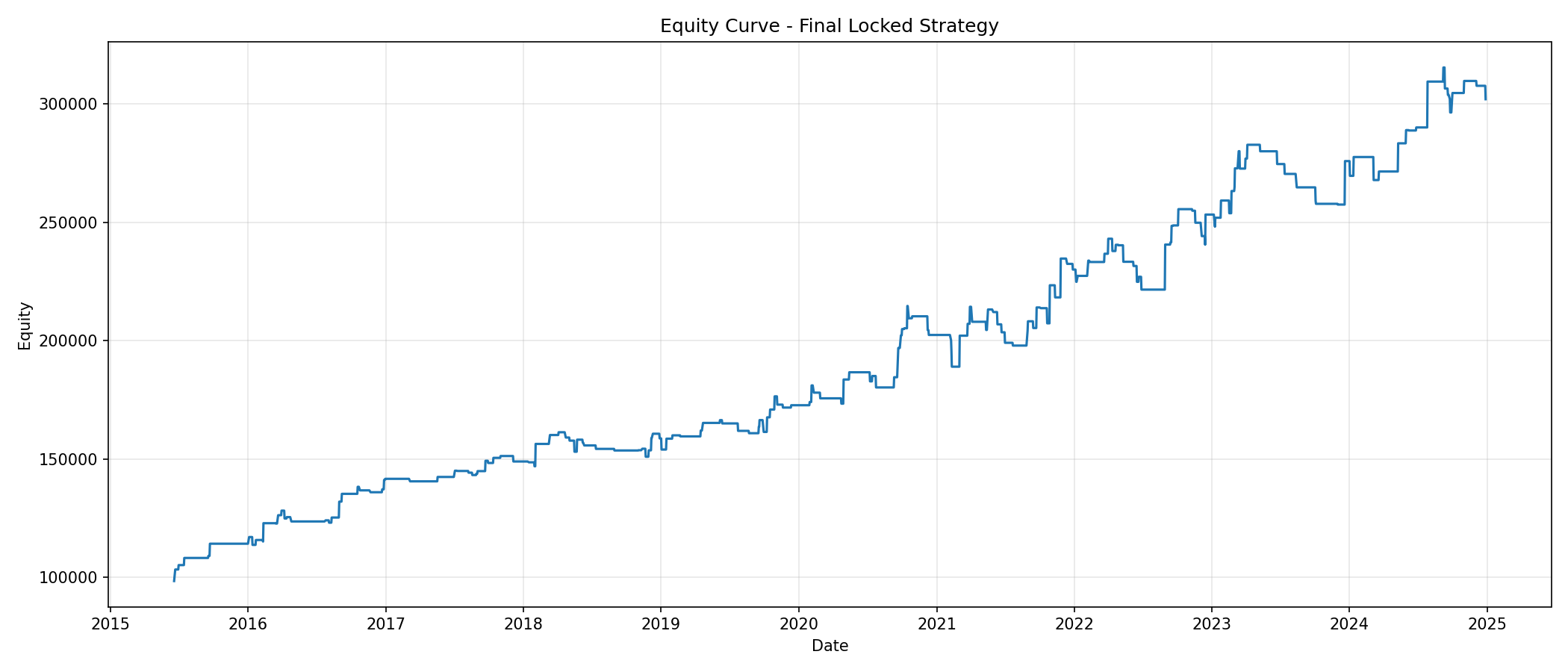
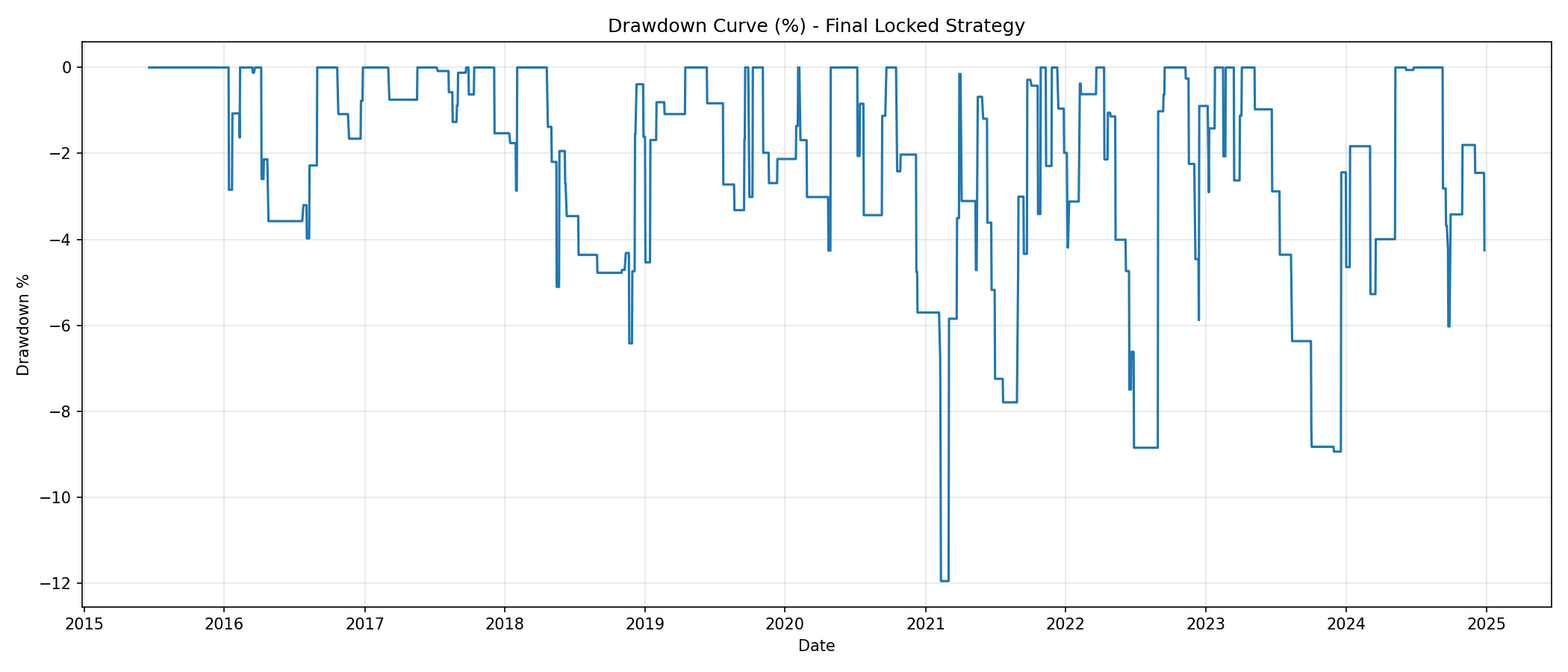
The equity curve climbs steadily but not smoothly. The deepest drawdown, about 12%, came in early 2021, and there were other extended flat or losing stretches in mid-2022 and late 2023. Every calendar year in the test ended positive, though 2017 and 2018 were thin.
| Year | Trades | Net PnL |
|---|---|---|
| 2015 (from June) | 6 | ₹14,146 |
| 2016 | 22 | ₹27,428 |
| 2017 | 13 | ₹7,327 |
| 2018 | 20 | ₹9,758 |
| 2019 | 19 | ₹14,022 |
| 2020 | 20 | ₹29,705 |
| 2021 | 25 | ₹27,637 |
| 2022 | 25 | ₹23,253 |
| 2023 | 19 | ₹22,607 |
| 2024 | 18 | ₹26,147 |
The strategy is very selective. Its filters let through roughly 20 trades a year, so a large share of trading days see no position at all.
Reading the Numbers Carefully: Capital Requirement
On the ₹1,00,000 base, net profit works out to a 202% return over about 9.5 years. The author flagged that this base isn’t one you could actually trade with.
Margin for one position (estimated at 15% of contract value) averaged ₹1,58,525 and peaked at ₹2,93,777 as NIFTY rose over the decade. A live account would need enough capital to cover peak margin plus a buffer for drawdowns. Here’s how the return changes with the capital assumption:
| Capital assumption | Capital base | Return on base |
|---|---|---|
| Nominal reporting base | ₹1,00,000 | 202.03% |
| Average margin per trade | ₹1,58,525 | 127.44% |
| Peak margin observed | ₹2,93,777 | 68.77% |
| Peak margin + maximum drawdown | ₹3,19,429 | 63.25% |
On the most realistic of these bases, the cumulative return over 9.5 years is about 63%, which is a CAGR of about 5.3% a year, compared with 12.30% on the nominal base. The Sharpe ratio and drawdown percentages above are also computed on the ₹1,00,000 base, so they would look more modest on a larger capital base too. This kind of adjustment is easy to skip, and it’s one of the more valuable parts of the project.
Where Did the Profit Come From? Exit Decomposition
Breaking the results down by exit type tells a story the summary table hides.
| Exit type | Trades | Win rate | Net PnL |
|---|---|---|---|
| Force exit (session close) | 99 | 86.87% | ₹4,10,202 |
| WMA trailing exit | 70 | 10.00% | -₹1,76,925 |
| Fixed stop-loss | 14 | 0.00% | -₹80,622 |
| 3R target hit | 4 | 100.00% | ₹49,373 |
More than half the trades ran all the way to the end-of-day square-off, and those trades produced all of the net profit and more. The WMA trailing exit, meant to protect gains, lost money overall with a 10% win rate. The 3R (1.5%) target was reached only four times in 187 trades.
In practical terms, the edge in this backtest comes from entering a confirmed intraday trend and holding it into the close. That has two implications. First, the trailing and target logic deserves its own review, since in this form it mostly cuts trades short. Second, anything that changes the end-of-day exit (broker auto square-off times, execution near the close, or rule changes) could materially change live results.
Key Observations
- The strategy combines indicator filters with session rules (opening-range check, lunch-hour block, late-entry cutoff and a daily loss cap). The session rules are design choices, and the project doesn’t isolate how much each one contributed.
- Combining Heikin Ashi candle structure with ADX/DMI filters kept the strategy very selective, at about 20 trades a year.
- The strategy stayed profitable in the backtest after slippage and costs, but those costs consumed a large share of gross profit.
- Profit depends heavily on holding trades to the close. The trailing exit was a net drag.
- Return figures depend on the capital base. On peak margin plus drawdown, the 9.5-year return is about 63% (about 5.3% CAGR), compared with 202% (12.30% CAGR) on the nominal base.
Limitations
Backtested results don’t predict live performance, and this project has several specific caveats:
- In-sample optimisation. Parameters were tuned and evaluated on the same 2015 to 2024 data. There’s no separate out-of-sample period yet, so some of the performance may reflect fitting to history.
- Small sample, many parameters. With 187 trades and more than a dozen tunable thresholds (WMA, RSI, ADX bands, DI gap, opening range, session times), overfitting risk is meaningful. The z-score of 2.77 says the average trade was positive in this sample, but it doesn’t correct for the number of parameter combinations tried.
- Untested session rules. The lunch-hour block and late-entry cutoff weren’t compared against versions of the strategy without them.
- Fixed quantity. The test trades 75 units throughout. That equalled one NIFTY lot only from late 2015 to mid-2021, so position sizing in a live setting would differ.
- Cost and margin assumptions. Slippage, charges and the 15% margin estimate are approximations. Real fills, especially near the close and in volatile sessions, may be worse.
- Data quality. Intraday futures data can contain gaps and irregular prints, and the way contract rollovers were handled in the source dataset can affect results.
Next Steps for the Strategy
The author suggests the following before considering any live use:
- A time-based train/test split, holding out the most recent years entirely.
- Rolling walk-forward validation to see whether the parameters hold across different market regimes.
- A separate review of the exit logic, testing variants with no trailing exit, a looser trail, or a stop that isn’t bound by the 0.5% minimum.
- Comparison runs with and without each session rule, to measure what each one adds.
- Position sizing that reflects actual exchange lot sizes and available capital.
- A period of paper trading to compare live fills against backtest assumptions.
Conclusion
This project builds a disciplined, multi-filter intraday trend-following system for NIFTY Futures and tests it with realistic costs and next-bar execution. The headline backtest numbers are positive, but the most instructive part of the work is how the author questioned them: recomputing returns on a deployable capital base and tracing the profit back to a single exit type. Those two checks turn a set of attractive metrics into a clear picture of what the strategy depends on and what still needs testing.
If you want to build and test strategies like this one, the Executive Programme in Algorithmic Trading (EPAT) covers Python for trading, backtesting, transaction-cost modelling and risk management, with a project component where participants work on their own strategy ideas under mentor guidance.
Bibliography
- Wilder, J. W. New Concepts in Technical Trading Systems.
- Chan, E. P. Algorithmic Trading: Winning Strategies and Their Rationale.
- Murphy, J. J. Technical Analysis of the Financial Markets.
- pandas documentation: https://pandas.pydata.org/
- NumPy documentation: https://numpy.org/
- NSE India market resources.
Download the Files
- Python notebook (NIFTY_HEKINASHI.ipynb)
- Trade log (trades_final.csv)
- Year-wise PnL (yearly_pnl_final.csv)
- Performance matrix (performance_matrix_final.csv)
Note: the raw NIFTY Futures data (sourced from TrueData) is not included. The notebook reads it from a local path, which readers will need to replace with their own data.
Disclaimer: The information in this project is true and complete to the best of our Student’s knowledge. All recommendations are made without guarantee on the part of the student or QuantInsti®. The student and QuantInsti® disclaim any liability in connection with the use of this information. All content provided in this project is for informational purposes only and we do not guarantee that by using the guidance you will derive a certain profit. Trading in futures involves substantial risk of loss and is not suitable for every investor.