The brass tacks of Julia programming

By Anshul Tayal

This is my second article in the Julia programming series. In my previous blog, I introduced you to Julia programming and discussed its origin and features. Here, I’ll work with the basic syntax of Julia programming.

I’ve divided this article into the following sections:

• Basic arithmetic operations
• General operations
• Strings
• Data structures
• Working with matrices
• Loops
• Conditional statements
• Functions
• Using R and Python code in Julia
• Python vs Julia - Comparison of syntax for basic operations

Let's start with the most traditional method of learning any new programming language.

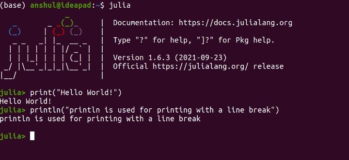
For the first few code snippets, I’ve deliberately used screen grabs from my Julia console so that you get a better feel of it.

Basic arithmetic operations

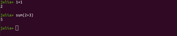
Let’s do some basic arithmetic operations using Julia. There are multiple ways of performing the same operation.

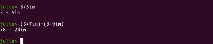
Here’s how you can write complex numbers and do basic operations on them.

When you add a floating-point number to an integer, it returns a floating-point number.

 ## Returns a float 
1.0 + 2 

Output: 3.0

Let’s look at division.

## Division 
1/2

Output: 0.5

Exponentiations can be done using the “^” symbol.

5^2

Output: 25

Julia can do operations on fractional numbers as well.

## Fractional numbers
1//2
## Adding fractional numbers
1//12 + 3//29

 Output: 65//348

General operations

Looking at the type of a variable is crucial while programming. Here’s how it can be done in Julia.

typeof(1)
typeof(1.0)
typeof('a')
typeof("Test")

Output:

Int64
Float64
Char
String

An important thing to note here is that characters are defined using single quotes while strings are defined using double quotes. A string in single quotes will return an error.

Let’s look at how to convert one variable type into another.

Converting a floating-point number into an integer.

# Method 1
convert(Int32, 1.0)

# Method 2
Int64(4.0)

Output:
1
4

The following example shows the method to comment multiple lines of code in Julia.

#=
Your comments here
Your comments here
Your comments here
=#

Single line comment can be written followed by “#”.

When you get stuck somewhere, the documentation can come in handy. Here’s how you can find out details of any function -

? log
Output: log(b,x) Compute the base blogarithm of x. Throws DomainError for negative Real arguments.
Examples
julia> log(4,8)
1.5
julia> log(4,2)
0.5

Strings

Now, let’s see how to use strings in Julia.

 "This is a string."

Output: This is a string.

Strings can be defined using "" or """ """. The use case for the second version would be when you need to use `` '' inside your string. For example -

 """ This is the use case for "triple-quote" string definition method.""" 

Output: This is the use case for \"triple-quote\" string definition method.

Here’s how we can use string-like variables.

variable = "Julia"
"This is how variables can be used inside strings in $variable."

Output: This is how variables can be used inside strings in Julia.

Exponentiation can be performed on strings as well. Here’s an example -

 variable^3 

Output: JuliaJuliaJulia

Let’s move on to the methods of manipulating strings. There are multiple ways of doing the same thing. Let’s look at how we can add 2 strings.

# Method 1

string("This is how we", " merge strings")
string("This is how we merge ", 2,  " strings with a number in-between")


# Method 2

var_1 = "This is method 2"
var_2 = "of concatenating strings in Julia"
var_1 * " " * var_2

# Method 3

var_3 = "This is method 3"
"$var_3 $var_2"

Output: 
This is how we merge strings 
This is how we merge 2 strings with a number in-between 
This is method 2 of concatenating strings in Julia 
This is method 3 of concatenating strings in Julia

Data structures

Data structures form the building blocks of any programming language. They provide different ways to organize the data in order to use them efficiently.

Tuples

Tuples are a type of data structure that can’t be modified. Here’s how you can define a tuple.

tuples = (1, 2, 3)
typeof(tuples)

Output:
(1, 2, 3)
Tuple{Int64, Int64, Int64}

Indexing in Julia starts at 1. Here’s how you can access the first and the last element of any data structure in Julia.

# Accessing the first element
tuples[1]

# Accessing the last element
tuples[end]

# [10] [11] Negative indexing doesn't work in Julia
tuples[-1]

# Tuples can't be modified
push!(tuples, 2)

Output:

1
3

BoundsError: attempt to access Tuple{Int64, Int64, Int64} at index [-1]
Stacktrace:
[1] getindex(t::Tuple, i::Int64)
@ Base ./tuple.jl:29
[2] top-level scope
@ In[30]:2
[3] eval
@ ./boot.jl:360 [inlined]
[4] include_string(mapexpr::typeof(REPL.softscope), mod::Module, code::String, filename::String)
@ Base ./loading.jl:1116
MethodError: no method matching push!(::Tuple{Int64, Int64, Int64}, ::Int64)
Closest candidates are:
push!(::Any, ::Any, ::Any) at abstractarray.jl:2387
push!(::Any, ::Any, ::Any, ::Any...) at abstractarray.jl:2388
push!(::AbstractChannel, ::Any) at channels.jl:10
...
Stacktrace:
[1] top-level scope
@ In[33]:2
[2] eval
@ ./boot.jl:360 [inlined]
[3] include_string(mapexpr::typeof(REPL.softscope), mod::Module, code::String, filename::String)
@ Base ./loading.jl:1116

Here’s how you can merge tuples -

# Concatenating tuples
(tuples..., tuples...)

# This method of adding "..." after any variable can be used to merge any two datatypes

Output:

(1, 2, 3, 1, 2, 3)

Vectors

Vectors are a type of data structure that can be modified. Here’s how you can work with vectors.

# Method 1
vector = [8, 1, 9, 12]

# Method 2
vector_2 = [8 ; 1 ; 9 ; 12]

Output:

4-element Vector{Int64}:

8
1
9
12

Here’s how mutation can be done in Julia. Using the “!” symbol, write the changes to the original variable. This is equivalent to “inplace=True” in Python.

# Mutation in Julia
sort(vector)

# The original vector doesn't change
sort!(vector)

# The original vector changes
vector

Output:

4-element Vector{Int64}:
1
8
9
12

To perform an element-wise operation, use the "." operator.

vector + 1 # This doesn't work

vector .+ 1

# Adding vectors
vector + vector_2

Output: 

4-element Vector{Int64}:
2
9
10
13

4-element Vector{Int64}:
2
16
18
24

Now, vectors can contain variables of different data types. Here’s an example -

vector_3 = [1, 5, "foo", 1+3im]

Output:

4-element Vector{Any}:
1
5
"foo"
1 + 3im

Notice that the vector type is assumed to be "Any" as there are variables of different data types.

Let’s look at the method of generating a sequence of numbers. Here’s an example of generating a sequence from 1 to 10 with a spacing of 2.

seq = [1:2:10;]

Here’s what the output looks like.

Output:

5-element Vector{Int64}:
1
3
5
7
9

Dictionaries

Now we move on to creating dictionaries. Dictionaries are used in a programming language to store information about a unique variable.

Just as each word in a human language dictionary has an associated meaning, in Julia we have each key that has a value associated with it.This can be useful in cases where you want to look up values associated with a particular key.

Here’s how you can create a dictionary in Julia.

dictionary = Dict('A' => 1, 'B' => 2)

This is what the output looks like -

Output:

Dict{Char, Int64} with 2 entries:
'A' => 1
'B' => 2

Now that we have created a dictionary, we would like to access various elements of it. Here’s how we can do it.

# Accessing the keys
keys(dictionary)

# Accessing the values associated with each key
values(dictionary)

Output:

KeySet for a Dict{Char, Int64} with 2 entries. Keys:
'A'
'B'

ValueIterator for a Dict{Char, Int64} with 2 entries. Values:
1
2

Let’s add a new entry to the dictionary.

# Adding a new entry

merge!(dictionary, Dict('J' => 23))

Output:

Dict{Char, Int64} with 3 entries:
'J' => 23
'A' => 1
'B' => 2

Notice that the “!” symbol makes the change permanent.

Let’s remove an entry now.

## Removing an entry permanently from a dictionary
pop!(dictionary, 'J')

dictionary

Output:

Dict{Char, Int64} with 2 entries:
'A' => 1
'B' => 2

Working with matrices

A matrix is an array of numbers represented as a vector of vectors. Here’s how you can create a matrix.

matrix_1 = [[1 2 3 ]; [4 5 6]]

Here’s what it looks like:

Output:

2×3 Matrix{Int64}:
1 2  3
4 5  6

Let’s look at various other operations in a matrix.

# Size of a matrix
print("This size of the matrix is" , size(matrix_1))

# Matrix
matrix_2 = [[2 2 0 ]; [2 7 9]]

#Transpose of a matrix
matrix_2'

# Accessing matrix elements
matrix_2[2,3]
matrix_2[1:4]

Output:

The size of the matrix is (2, 3)

2×3 Matrix{Int64}:
2 2  0
2 7  9

9

4-element Vector{Int64}:
2
2
2
7

Let’s add and multiply matrices now.

# Adding matrices
matrix_2 + matrix_1
matrix_3 = [[2 3] ; [5 6] ; [4 5]]

# Multiplying matrices
matrix_1 * matrix_3

The output of addition is -
2×3 Matrix{Int64}:
3 4   3
6 12  15

The output of multiplication is -
2×2 Matrix{Int64}:
24  30
57  72

Performing the elementwise operation in Julia using the "." symbol. Any operation followed by "." will perform. Here’s an example of taking the log of each element of a matrix. It is equivalent to the map() function in Python

# element wise operation.

log.(matrix_1)

Output:

2×3 Matrix{Float64}:
0.0 0.693147  1.09861
1.38629 1.60944   1.79176

Let’s create a matrix with zeros and ones. You can use the function zeros() and ones() to do that.

zero = zeros(3,4)
one = ones(2,3)

Output:

3×4 Matrix{Float64}:
0.0 0.0  0.0  0.0
0.0 0.0  0.0  0.0
0.0 0.0  0.0  0.0

2×3 Matrix{Float64}:
1.0 1.0  1.0
1.0 1.0  1.0

Let’s see how to generate random values.

rand_1 = rand(5)

# Random values in 2D
rand_2 = rand(5, 2)

# Random values in 3D
rand_3 = rand(3, 2, 2)

Output:

5-element Vector{Float64}:
0.24942793903668203
0.8454642816997531
0.8538602946052574
0.21154126925067507
0.07873330355017316

5×2 Matrix{Float64}:
0.706975 0.935989
0.494324 0.988657
0.994824 0.943832
0.44183 0.404011
0.802337 0.124313

3×2×2 Array{Float64, 3}:
[:, :, 1] =
0.443337 0.813706
0.958816 0.53124
0.203751 0.951473

[:, :, 2] =
0.125259 0.761672
0.440907 0.0505402
0.161741 0.672215

Loops

A loop helps in performing the same task repeatedly.  There are multiple types of loops used in programming . Mostly, they are:

• For loop - This type of loop is used when the no. of iterations to be run are known beforehand.
• While loop - This type of loop is used when the no. of iterations depends on a condition.

Let’s see how to create them in Julia.

## While loop

var = 0
while var < 10
var += 1
println(var)
end

Output:

1
2
3
4
5
6
7
8
9
10

## For loop

# Method 1
for i in 1:10
println(i)
end

# Method 2
colleagues = ["Vivek", "Jay", "Mario", "Udisha"]
for colleague in colleagues
println(colleague)
end

# Method 3
c = [i+j for i in 1:3, j in 1:5]

Output:

The output of method 1 -
1
2
3
4
5
6
7
8
9
10

The output of method 2 -
Vivek
Jay
Mario
Udisha

The output of method 3 -
3×5 Matrix{Int64}:
2 3  4  5  6
3 4  5  6  7
4 5  6  7  8

There are multiple methods of performing the same operations in any programming language. Feel free to take your own approach.

Conditional statements

Let’s move on to the conditional statements. These are if-else conditional statements where you want to perform an operation when a certain event occurs. Here’s the control flow.

Here’s the syntax -

if condition 1
println(“Statements if condition 1 is true”)
else
println(“Statements if condition 1 is false”)
end

Here’s how you can do it.

var_1 = 31
var_2 = 45

# Method 1
if var_1 > var_2
println("$var_1 is larger than $var_2")
elseif var_2 > var_1
println("$var_2 is larger than $var_1")
else
println("None")
end

# Method 2
# condition ? True:False
(var_1 > var_2) ? var_1 : var_2

# Method 3
# && is logical "and" operator
(var_1 > var_2) && [22] println("$var_1 is larger than $var_2")
(var_2 > var_1) && println("$var_2 is larger than $var_1")

Output:

45 is larger than 31

45

false

45 is larger than 31

Functions

Functions are a set of instructions written together so that they can be used multiple times without writing the code repeatedly.

Creating functions also helps debug the code easily as you can look at individual blocks (functions) and figure out the one with the error.

Here’s how we can write functions in Julia:

# Method 1
function power_5(var_1)
return var_1^5
end

# Calling the function
power_5(4)

# Method 2
power_5(x) = x^5
power_5(4)

Output:

1024
1024

Using R and Python code in Julia

There can be times where you want to use your R or Python code as the libraries to perform certain operations may not be available in Julia.

However, using 2 languages to perform a certain operation can be a challenge. Hence, Julia provides an option to use R and Python code by using the “PyCall” and “RCall” packages.

How to use Python code in Julia

Here’s how you can use your Python code in Julia.

# Install the "PyCall" package for Python
using Pkg
Pkg.add("PyCall")
using PyCall

## Importing numpy package from Python
np = pyimport("numpy")

## Using numpy package in Julia
np.array([1,2,3])

Output:

3-element Vector{Int64}:
1
2
3

How to use R code in Julia

Let’s look at an example of using R in Julia.

# Install "RCall" package for R
Pkg.add("RCall")
using RCall

# There are several ways to call R code

# Method 1
# Calling the mean() function from R
rcall(:mean, [1,2,3])

# Method 2 for user-defined functions
R"""
power_4 <- function(x)
{
return(x^4)
}"""
    
## Calling the defined function
rcall(:power_4, 5)

Output:

RObject{RealSxp}
[1] 2
RObject{RealSxp}
[1] 625

For further details on using the RCall package, you can refer here.

Python vs Julia - Comparison of syntax for basic operations

Conclusion

In this article, we went through the code snippets to get started. The idea was to introduce you to the basic syntax and the possibilities of this programming language.

The next article will introduce you to the data visualization techniques in Julia. Until then, feel free to explore and create your own Julia journey!

However, if you looking to pursue and venture into algorithmic trading then our comprehensive algo trading course taught by industry experts, trading practitioners and stalwarts like Dr. E. P. Chan, Dr. Euan Sinclair to name a few - is just the thing for you. Enroll now!

Disclaimer: All data and information provided in this article are for informational purposes only. QuantInsti^® makes no representations as to accuracy, completeness, currentness, suitability, or validity of any information in this article and will not be liable for any errors, omissions, or delays in this information or any losses, injuries, or damages arising from its display or use. All information is provided on an as-is basis.