
In the last blog, we examined the steps to train and optimize a classification model in scikit learn. In this blog, we bring our focus to linear regression models. We will discuss the concept of regularization, its examples (Ridge, Lasso and Elastic Net regularizations) and how they can be implemented in Python using the scikit learn library.
Content
- Importing Libraries
- The Data: "diabetes" Dataset from Scikit Learn
- Data Preprocessing
- Model Evaluation Metric
- Simple Linear Regression
- Multiple Linear Regression
- Why Regularize?
- What is Ridge Regression?
- Implementing Ridge Regression in scikit learn
- What is Lasso Regression?
- What is Elastic Net Regression?
- Summary
Linear Regression problems also fall under supervised learning, where the goal is to construct a "model" or "estimator" which can predict the continuous dependent variable(y) given the set of values for features(X).
One of the underlying assumptions of any linear regression model is that the dependent variable(y) is (at least to some degree!) a linear function of the independent variables(Xis). That is, we can estimate y using the mathematical expression:
\(y = b_0 + b_1 X_1 + b_2 X_2 + b_3 X_3 + \cdots+ b_n X_n\) ,
where, \(b_i\)s are the coefficients that are to be estimated by the model.
The cost function that we seek to minimize is the sum of squared errors(also referred to as residuals). This methodology is called the ordinary least squares(OLS) approach. In other words, we want those optimal values of bis that minimize \( \sum (y - \hat{y})^2\ \), where \(\hat{y}\) is the value of y predicted by the model.
Although the OLS approach works well in a lot of cases, it has its own drawbacks when the data has far-flung outliers or when the predictor variables (\(X_i\)s) are correlated with each other.
This can have a significant impact on the overall prediction accuracy of the model, especially for out of sample or new data. In such cases, some form of regularization is helpful.
Two of the most popular regularization techniques are Ridge regression and Lasso regression, which we will discuss in this blog.
Let us begin from the basics, i.e. importing the required libraries.
Importing Libraries
We will need some commonly used libraries such as pandas, numpy and matplotlib along with scikit learn itself:
That's it!
In the next section, we will get some data to build our models on.
The Data: "diabetes" Dataset from Scikit Learn
Scikit learn comes with some standard datasets, one of which is the 'diabetes' dataset.
In this dataset, ten baseline variables(features), age, sex, body mass index, average blood pressure, and six blood serum measurements(s1, s2, s3, s4, s5 and s6) were obtained for each of 442 diabetes patients, along with response of interest, a quantitative measure of disease progression (y) one year after baseline.
This dataset represents a classic regression problem, where the challenge is to model response y based on the ten features. This model can then be used for two purposes:
- one, to identify the important features (out of the ten mentioned above) that contribute to disease progression
- and two, to predict the response for future patients based on the features
Each of these ten feature variables has been mean-centred and scaled by the standard deviation times n_samples (i.e. the sum of squares of each column totals 1)
Check out https://scikit-learn.org/stable/datasets/index.html for more information, including the source URL.
Let us get the diabetes dataset from the "datasets" submodule of scikit learn library and save it in an object called "diabetes" using the following commands:
We now have loaded the data in the "diabetes" object. But in order to train models on it, we first need to get it in a format that is conducive and convenient for this process. In the next step, we do just that.
Data Preprocessing
The "diabetes" object belongs to the class Bunch, i.e. it is a collection of various objects bunched together in a dictionary-like format.
These objects include the feature matrix "data" and the target vector "target". We will now create a pandas dataframe containing all the ten features and the response variable (diab_measure) using the following commands:
Output:
| age | sex | bmi | bp | s1 | s2 | s3 | s4 | s5 | s6 | diabetes_measure | |
|---|---|---|---|---|---|---|---|---|---|---|---|
| 0 | 0.038076 | 0.050680 | 0.061696 | 0.021872 | -0.044223 | -0.034821 | -0.043401 | -0.002592 | 0.019908 | -0.017646 | 151.0 |
| 1 | -0.001882 | -0.044642 | -0.051474 | -0.026328 | -0.008449 | -0.019163 | 0.074412 | -0.039493 | -0.068330 | -0.092204 | 75.0 |
| 2 | 0.085299 | 0.050680 | 0.044451 | -0.005671 | -0.045599 | -0.034194 | -0.032356 | -0.002592 | 0.002864 | -0.025930 | 141.0 |
| 3 | -0.089063 | -0.044642 | -0.011595 | -0.036656 | 0.012191 | 0.024991 | -0.036038 | 0.034309 | 0.022692 | -0.009362 | 206.0 |
| 4 | 0.005383 | -0.044642 | -0.036385 | 0.021872 | 0.003935 | 0.015596 | 0.008142 | -0.002592 | -0.031991 | -0.046641 | 135.0 |
All the features and the response variable are now in a single dataframe object. In the next step, we will create the feature matrix(X) and the response variable(y) using the dataframe we just created:
Now that we have our feature matrix and the response vector, we can move on to build and compare different regression models. But in order to do that, we first need to choose a suitable methodology to evaluate and compare these models. In the next section, we do just that.
Model Evaluation Metric
Scikit learn provides a varied list of scoring metrics to evaluate models. As we will be comparing linear regression models today, the 'neg_mean_squared_error' is the most suited for us.
The general convention followed by all the metrics in scikit learn is that higher return values are better than lower return values.
Thus metrics which measure the distance between the predicted model values and the actual data values(like metrics.mean_squared_error) are available as neg_mean_squared_error. So, for example, a model with -100 neg_mean_squared_error is better than the one having -150 neg_mean_squared_error.
You can check out the whole list of scoring metrics using the command:
Simple Linear Regression
The simplest form of linear regression is where there is only one feature of a predictor variable/feature. We often hear that a healthy BMI (Body Mass Index) ratio is conducive to a lower chance of developing a diabetic condition.
We can quantify this relation using a simple linear regression model. But first, we need to fetch and save the feature 'BMI' and the response variable 'diabetes_measure' in a form that can be used in scikit learn as follows:
The steps to building a machine learning model pretty much remain the same as discussed in the previous blog on classification models. Let us build a simple linear regression model to quantify the relationship between BMI and diabetes, based on the data we have:
The object 'predicted_y' contains all the response values predicted by our model 'simple_lr'.
Let us now plot the regression line for our model to get a visual representation:
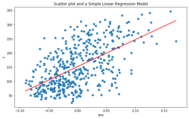
In the above plot, the blue dots are the actual data points (x,y). Visually, there seems to be a positive linear relationship between BMI(Body mass index) and the diabetes measure(y), that our model (red line) is trying to capture. But how good is it in doing so?
In the previous blog, we have also discussed the concepts related to k-fold cross-validation, that we will apply here. The 'cross_val_score' function from the model_selection submodule of scikit learn, takes in an estimator(model) object, a feature matrix, a response vector, a scoring mechanism ('neg_mean_squared_error' in our case) and cv as parameters.
Setting a value of cv to 10, means 10-fold cross-validation will be performed on the given data using the given estimator and corresponding ten 'neg_mean_squared_errors' scores will be generated.
We will simply use the mean of all these ten scores (mse) as an indicator of how good the model is.
Thus we have an average score of -3906.92 for 'neg_mean_squared_error' for our simple linear regression model 'simple_lr'.
Let us check if adding more features improves model considerably producing an overall better average score. This means we are seeking to build a linear regression model with multiple features, also called multiple linear regression, which is what we do next.
Multiple Linear Regression
The basic steps will remain the same as the previous model, with the only difference being that we will use the whole feature matrix X (all ten features) instead of just one feature:
Output:
We see that adding the nine remaining features to the model along with bmi, increases the average 'neg_mean_squared_error' from almost -3906.92 to about -3000.38, which is a considerable improvement.
Let us take a look at all the ten coefficient values for the 'multiple_lr' model using the following command:
Output:
Note that none of the estimated coefficient values are 0. Plotting the above values along with the corresponding feature names on the x-axis using the commands from the matplotlib library:
Output:
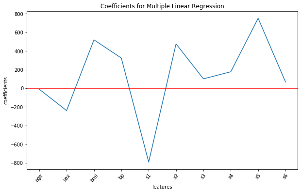
We see that in this model, the features bmi, s1, s2 and s5 are having a considerable impact on the progression of diabetes, as all of them have high estimated coefficient values.
Why Regularize?
One of the basic assumptions of a multiple linear regression model is that there should be no (or very less) multicollinearity among the feature variables. This essentially means that the feature variables should ideally have no or very less correlation with each other.
A high correlation between the two feature variables gives rise to several problems. If we include one of them in the model, adding the other will have little or no impact on improving the model, but will only make the model more complex.
This goes against the principle of 'parsimony' in model building, which dictates that a simpler model with fewer variables is always preferred to a more complex model with too many features.
In such a case the whole OLS model becomes less reliable as the coefficient estimates have high variance, i.e. they do not generalize well to unseen data(also called the problem of overfitting).
The correlations among all the feature variables can be visualized with the help of a correlation matrix using the following commands:
Output:
| age | sex | bmi | bp | s1 | s2 | s3 | s4 | s5 | s6 | |
|---|---|---|---|---|---|---|---|---|---|---|
| age | 1 | 0.173737 | 0.185085 | 0.335427 | 0.260061 | 0.219243 | -0.075181 | 0.203841 | 0.270777 | 0.301731 |
| sex | 0.173737 | 1 | 0.0881614 | 0.241013 | 0.0352768 | 0.142637 | -0.37909 | 0.332115 | 0.149918 | 0.208133 |
| bmi | 0.185085 | 0.0881614 | 1 | 0.395415 | 0.249777 | 0.26117 | -0.366811 | 0.413807 | 0.446159 | 0.38868 |
| bp | 0.335427 | 0.241013 | 0.395415 | 1 | 0.24247 | 0.185558 | -0.178761 | 0.257653 | 0.393478 | 0.390429 |
| s1 | 0.260061 | 0.0352768 | 0.249777 | 0.24247 | 1 | 0.896663 | 0.0515194 | 0.542207 | 0.515501 | 0.325717 |
| s2 | 0.219243 | 0.142637 | 0.26117 | 0.185558 | 0.896663 | 1 | -0.196455 | 0.659817 | 0.318353 | 0.2906 |
| s3 | -0.075181 | -0.37909 | -0.366811 | -0.178761 | 0.0515194 | -0.196455 | 1 | -0.738493 | -0.398577 | -0.273697 |
| s4 | 0.203841 | 0.332115 | 0.413807 | 0.257653 | 0.542207 | 0.659817 | -0.738493 | 1 | 0.617857 | 0.417212 |
| s5 | 0.270777 | 0.149918 | 0.446159 | 0.393478 | 0.515501 | 0.318353 | -0.398577 | 0.617857 | 1 | 0.46467 |
| s6 | 0.301731 | 0.208133 | 0.38868 | 0.390429 | 0.325717 | 0.2906 | -0.273697 | 0.417212 | 0.46467 | 1 |
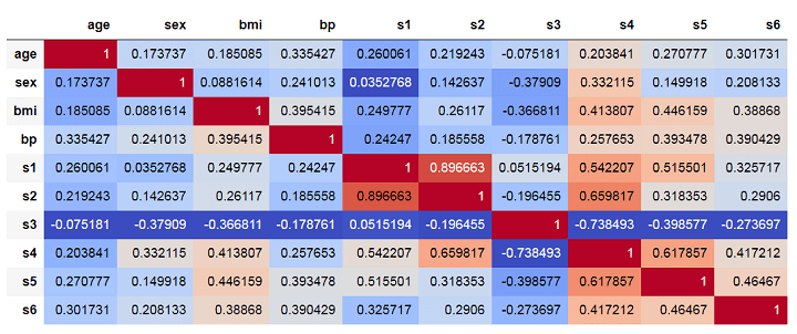
The above matrix shows correlations among the features such that darker shades of red implying high positive correlation and darker shades of blue implying high negative correlations.
In the multiple linear models we built in the previous section, both features s1 and s2 came out as important features. However, we can see that they have a very high positive correlation of about 0.896. This is clearly inducing multicollinearity into the model.
To counter such issues, we can use regularization techniques which allow us to lower this variance of the model at the cost of adding some bias into it, such that the total error is reduced. Lower variance implies that the problem of overfitting is tackled automatically, as the model generalizes well to unseen data after regularization.
The regularization techniques work by adding penalty factors to the original OLS cost function such that high coefficient values are penalized, taking them closer to zero.
The features with significant coefficient values are identified after a regularization procedure and other insignificant features with near-zero coefficient values can be dropped. This also leads to what is called natural features selection, resulting in an overall parsimonious model.
There are many regularization techniques, of which we discuss the three most commonly used ones viz. Ridge, Lasso and Elastic Net in the upcoming sections.
What is Ridge Regression?
Ridge regression (often referred to as L2 regularization) is a regularization technique in which the aim is to find those optimal coefficient estimates that minimize the following cost function:
OLS cost function + Penalty for high coefficient estimates = \( \sum (y - \hat{y})^2\ \) + \(alpha \cdot (b1^2+\cdots+bk^2)\).
Here, alpha is the hyperparameter representing regularization strength. A high value of alpha imposes a high penalty on the sum of squares of coefficient estimates.
The value of alpha can be any positive real number value. When alpha is 0, it is same as performing a multiple linear regression, as the cost function is reduced to the OLS cost function.
Implementing Ridge Regression in scikit learn
As alpha is a hyperparameter, its optimal value (that maximizes average neg_mean_squared_error for the model) can be found using the GridSearchCV algorithm in scikit learn as follows:
We see that regularizing our multiple linear regression model using Ridge regression, increases the average 'neg_mean_squared_error' from almost -3000.38 to about -2995.94, which is a moderate improvement.
Let us visualize all the ten coefficient estimates for the ridge regression model using the following commands:
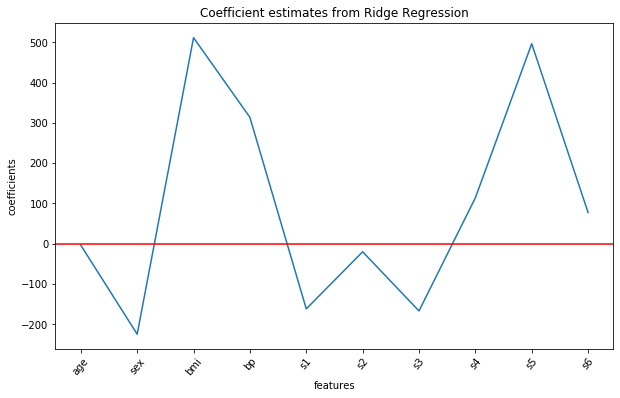
Previously, features s1 and s2 came out as an important feature in the multiple linear regression, however, their coefficient values are significantly reduced after ridge regularization. The features 'bmi' and s5 still remain important.
What is Lasso Regression?
Lasso regularization (called L1 regularization) is also a regularization technique which works on similar principles as the ridge regularization, but with one important difference. The penalty factor in Lasso regularization is composed of the sum of absolute values of coefficient estimates instead of the sum of squares.
Thus, the aim in Lasso regression is to find those optimal coefficient estimates that minimize the following cost function :
OLS cost function + Penalty for high coefficient estimates = \( \sum (y - \hat{y})^2\ \) + \(alpha \cdot (|b1|+\cdots+|bk|)\).
Note that in the case of Lasso, the penalty is made up of the sum of absolute values (i.e. magnitudes) of coefficients, unlike in Ridge regression (where it was made up of the sum of squares instead).
Here, alpha is still the hyperparameter representing regularization strength. A high value of alpha imposes a high penalty on the sum of magnitudes of coefficient estimates. The value of alpha can be any positive real number value as before.
We can use the following commands to get the optimal value of alpha in case of Lasso regression using the GridSearchCV algorithm:
We see that using Lasso regularization produces slightly better results as compared to the Ridge regularization, i.e. increases the average 'neg_mean_squared_error' from almost -3000.38 to about -2986.37 (compared to -2995.94 from Ridge regularization).
Let us visualize all the ten coefficient estimates for the Lasso regression model using the following commands:
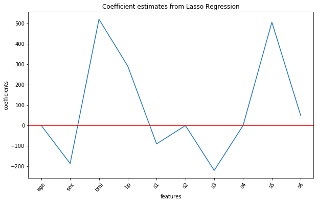
Output:
Lasso regularization completely eliminates features 'age', s2 and s4 from the model (as their estimated coefficients are 0) and gives us a parsimonious model (simpler model with less variables) with overall best score.
What is Elastic Net Regression?
Elastic Net regularization combines the power of Lasso and Ridge regularizations into one single technique. The cost function to be minimized for Elastic Net is :
OLS cost function + Lasso Penalty term + Ridge Penalty term =
\( \sum (y - \hat{y})^2\ + alpha \cdot(l1\_ratio) \cdot (|b0| + |b1|+\cdots+|bk|) + alpha \cdot(1- l1\_ratio) \cdot (b0^2 + b1^2+\cdots+bk^2)\).
The above cost function has two important hyperparameters: alpha and l1_ratio. Alpha in case of Elastic Net regularization is a constant that is multiplied with both L1(Lasso) and L2(Ridge) penalty terms. The hyperparameter l1_ratio is called the mixing parameter such that 0 <= l1_ratio <= 1.
When l1_ratio is 1, it means that the share of L1 (Lasso) is 100% and that of L2 (Ridge) is 0%, i.e. same as a Lasso regularization. Similarly, when l1_ratio is 0, it is same as a Ridge regularization.
The optimal values for both alpha and l1_ratio can be determined using GridSearchCV algorithm as follows:
Let us now take a peek at the best values for hyperparameters alpha and l1_ratio (and the best score from Elastic Net regularization):
Output:
Output:
In this case, the best l1_ratio turns out to be 1, which is the same as a Lasso regularization. Consequently, the best score also remains the same as obtained from Lasso regularization earlier.
Summary
Let us compare the coefficient estimates obtained from:
- Multiple linear regression without any regularization
- Ridge regularization and
- Lasso regularization
Note that in this case, the resulting estimates from Elastic Net regularization were exactly the same as Lasso and hence we will not consider it separately.
The following code puts coefficient estimates from all the three models side by side in a dataframe format:
Output
| without_regularization | Ridge | Lasso | |
|---|---|---|---|
| age | -10.0122 | -3.60965 | -0 |
| sex | -239.819 | -224.329 | -186.309 |
| bmi | 519.84 | 511.204 | 520.894 |
| bp | 324.39 | 313.553 | 291.196 |
| s1 | -792.184 | -161.534 | -90.0686 |
| s2 | 476.746 | -19.893 | -0 |
| s3 | 101.045 | -166.68 | -220.207 |
| s4 | 177.064 | 113.95 | 0 |
| s5 | 751.279 | 496.222 | 506.422 |
| s6 | 67.6254 | 77.4439 | 49.0746 |
Also we can plot the coefficient values from all the three models on the same plot for visual comparison as follows:

We can observe the following general points about Ridge and Lasso regularizations clearly:
- Although Ridge regularization shrinks the values of coefficient estimates considerably by pulling them closer to zero, it does not make them exactly zero.
- On the other hand, Lasso regularization completely eliminates features ('age', 's2' and 's4' in our example) from the model by assigning their coefficients zero values. This results in a much more parsimonious/more simple model.
Also, Lasso regularization produces the best average score (-2986.36) out of all the three models. Thus, Lasso regularization is the clear winner in this case, as it yields the best average score and also gives a smaller/simpler model. However, this is not always the case.
Lasso regularization tends to perform better in a case where a relatively small number of features have substantial coefficients (such as bmi and s5 in our example).
On the other hand, Ridge regression performs better in a case where the coefficients are roughly of equal size, i.e. all the features impact the response variable somewhat equally.
Conclusion
This brings us to the end of yet another blog on model building and fine-tuning in scikit-learn. Hopefully, you have enjoyed reading this blog and picked up a few useful points from it.
In the next few blogs, we will shift our focus onto other machine learning algorithms, the intuitions behind why they work and how to implement them practically in Python.
Happy learning till then!
If you too desire to equip yourself with lifelong skills which will always help you in upgrading your trading strategies. With topics such as Statistics & Econometrics, Financial Computing & Technology, Machine Learning, this algo trading course ensures that you are proficient in every skill required to excel in the field of trading. Check out EPAT now!
Disclaimer: All investments and trading in the stock market involve risk. Any decisions to place trades in the financial markets, including trading in stock or options or other financial instruments is a personal decision that should only be made after thorough research, including a personal risk and financial assessment and the engagement of professional assistance to the extent you believe necessary. The trading strategies or related information mentioned in this article is for informational purposes only.
