
As trading becomes automated, we have seen that traders seek to use as much data as they can for their analyses. But we all know that adding more variables leads to more complications and that in turn might make it harder to come to solid conclusions. Think about it, we have more than 3000 companies in the New York Stock Exchange. A simple exercise to find pairs between them will be really computing-intensive. Wouldn’t it be wonderful if we could use a lot of variables but still somehow make it simpler?
Well, worry not my friend. We have the answer, or rather, Principal Component Analysis is the answer.
If we had to describe the usefulness of Principal Component Analysis, we would say that it helps us reduce the amount of data we have to analyse. Don’t worry if you are still confused. We will go through the following topics in this blog.
- What is Principal Component Analysis?
- Eigen Vectors and Covariance Matrix
- When to use Principal Component Analysis?
- Principal Component Analysis in trading
What is Principal Component Analysis?
Principal Component Analysis is one of the methods of dimensionality reduction and in essence, creates a new variable which contains most of the information in the original variable. An example would be that if we are given 5 years of closing price data for 10 companies, ie approximately 1265 data points * 10. We would seek to reduce this number in such a way that the information is preserved.
Of course, in the real world, there would be some information loss and thus, we use the principal component analysis to make sure that it is kept to a minimum.
That sounds interesting, but how do we do this exactly?
The answer is EigenValues. Well, that’s not the whole answer but in a way it is. Before we get into the mathematics of it, let us refresh our concepts about the Matrix (no, not the movie!). If you want to skip the refresher, click on this link to move ahead.
Eigen Vectors and Covariance Matrix
One of the major applications of Eigenvectors and Eigenvalues is in image transformations. Remember how we can tilt an image in any of the photo editing apps. Well, Eigenvalues and Eigenvectors helps us in this regard.
Basically, when we multiply a vector with a matrix the vector gets transformed. By transformed we mean the direction and the magnitude of the vector might change. There are however some vectors for which the direction does not change. The magnitude might change however. So formally, this is what happens, for a transforming matrix A and a vector v:
Av = λv
The entire set of such vectors which do not change direction when multiplied with a matrix are called Eigen Vectors. The corresponding change in magnitude is called the Eigen Value. It is represented with λ here.
Remember how we said that the ultimate aim of the principal component analysis is to reduce the number of variables. Well, Eigenvectors and Eigenvalues help in this regard. One thing to follow is that Eigenvectors are for a square matrix i.e. a matrix with an equal number of rows and columns. But they can also be calculated for rectangular matrices.
Let’s say we have a matrix A, which consists of the following elements:
|
2 |
8 |
|
6 |
10 |
Now, we have to find the Eigenvectors and Eigenvalues in such a manner such that:
Av = λv
Where,
v is a matrix consisting of Eigenvectors, and
λ is the Eigenvalue
While it may sound daunting, but there is a simple method to find the Eigenvectors and Eigenvalues.
Let us modify the equation to the following,
Av = λIv (We know that AI = A)
If we bring the values from the R.H.S to the L.H.S, then,
Av - λIv = 0
Now, we will assume that the Eigenvector matrix is non-zero. Thus, we can find λ by finding the determinant.
Thus, | A - λI | = 0
(2 - λ)(10 - λ) - (8*6) = 0
20 - 2λ - 10λ +λ^2 - 48 = 0
-28 -12λ+ λ^2 = 0
λ^2 -12λ - 28 = 0
(λ - 14)(λ +2) = 0
λ = 14, -2
Thus, we can say that the Eigenvalues are 14, -2.
Taking the λ value as -2. We will now find the Eigenvector matrix.
Recall that, Av = λv
Let’s say that the Eigenvector matrix is as follows:
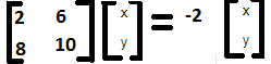
(2x + 6y) = -2x
(8x + 10y) = -2y
(4x + 6y) = 0
(8x + 12y) = 0
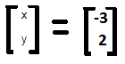
Since they are similar, solving them to get, 2x + 3y = 0, x = (-3/2)y
X = -3, y = 2
Thus, the Eigenvector matrix is
The entire equation can now be written in the following manner,
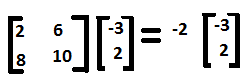
Similarly, for λ = 14, the Eigenvectors are x =1, y = 2
That’s awesome! We have understood how Eigenvectors and Eigenvalues are formed. Hold on, let’s ask ourselves a simple question, between the two sides of the equation, does L.H.S look simple or R.H.S?
Now that we know how to find the Eigenvalues and Eigenvectors, let us talk about their properties.
In our earlier example, we had a 2 x 2 matrix. This can be considered as 2 dimensions. One of the great things about Eigenvectors and Eigenvalues is that they are used for “Orthogonal transformations” which is a fancy word for saying that the variables are shifted in another axis with changing the direction. Let us take a visual example of this.
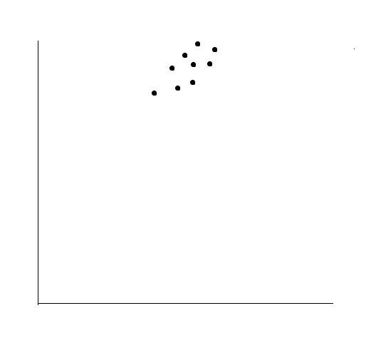
Let’s say we have the following values mapped on the x and y axis. Now you can locate them by giving the (x,y) coordinates of a point but we realise that there can be another efficient way to display them meaningfully.
What if we draw a line in such a way that we can locate them using just the distance between a point on this new line and the points. Let’s try that now.
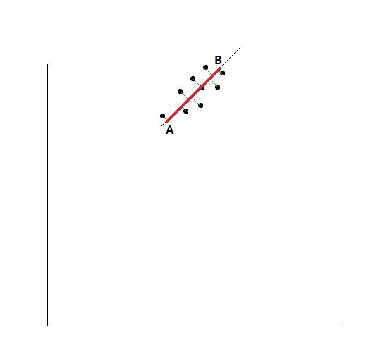
Let us say that the green lines represent the distance from each point to the new line. Furthermore, the distance from the first point on the line projected, to the last point’s projection on the new line is referred to as the spread here. In the above figure, it is denoted as the red line. The importance of spread is that it gives us information on how varied is the data set. The larger the value, the easier it is for us to differentiate between two individual data points.
We should note that if we had variables in two dimensions, then we will get two sets of Eigenvalue and Eigenvectors. The other line would actually be perpendicular to the first line.
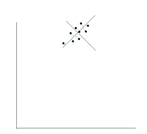
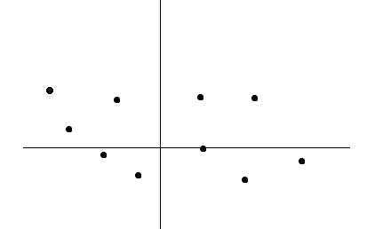
Now, we have a new coordinate axis which is much more suited to the points, right?
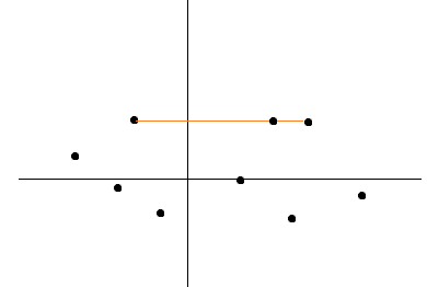
Let’s plot the variable according to the new axis.
If we had to explain Eigenvectors and Eigenvalues diagrammatically, we can say that the Eigenvectors gives us the direction in which it is stretched or transformed and the Eigenvalues is the value by which it is stretched. In that sense, the first line gives us more information when it comes to the spread than the second line.
But why is this important to understand. When we said the Eigenvalues gives us the value by which the points are stretched, we should add further that the Eigenvalues with the corresponding larger number gives us more information than the one with the lesser valued Eigenvalue.
Oh, wait! This article talks about Principal Component Analysis. Well, the Eigenvalues and Eigenvectors are actually the components of the data.
But there is one missing part of the puzzle left. As we have seen the illustration, the data points were bunched together, and hence the distance between the points was not that significant.
But what if we were trying to compare stock prices, one whose value was less than $10 and another which was more than $500? Obviously, the variation in the price itself would lead to a different result. Hence, we try to find a way to standardise the data. And since we are trying to find the difference, what better way than to use the covariance matrix.
Covariance
Covariance is essentially used to see the direction in which two corresponding variables move. Let us quickly explain covariance with a real-world example.
Covariance using stock data
Let us say that the ‘n’ stocks in our portfolio (S1, S2,…Sn) have closed price as given below

We will combine this stock data in a single matrix and name it as 'S':

Average Price Of Stock
As you can see each stock consists of the past ‘m’ days close prices. Using this data, we will first compute the average price for each stock.
For example, the mean price for stock 'S1' is given as follows:
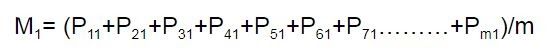
Next, we save all the means of 'n' stocks in a matrix called 'M' as follows:

Our ultimate aim is to understand how one stock’s behaviour is related to that of another’s. To compare two stocks with two completely different price ranges, we need to first establish a common base. So to make the comparison of stocks movements even, we subtract the mean of the stock price from the stock price.
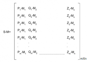
This will create a new de-meaned stock price which will help in comparing how one stock's movement from its mean is dependent on another’s movement from it’s mean. Let us understand how to create a de-meaned series.
Demeaning The Prices
First, we subtract the mean stock price from the close prices of the corresponding stock. This will give us the matrix with de-meaned scores, or a measure of how far a data point is from its mean.
Covariance Matrix
Once we have the de-meaned price series, we establish the covariance of different stocks by multiplying the transpose of the de-meaned price series with itself and divide it by 'm' (number of data points), this gives us the covariance matrix:
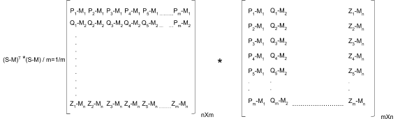

In the resulting covariance matrix, the diagonal elements represent the variance of the stocks.
Also, the covariance matrix is symmetric along the diagonal, meaning:
σ21 = σ12
Thus, in this manner, we can find the variance as well as the covariance of a dataset. If you are interested in portfolio variance, then head on over to this blog. The above definition of co-variance is taken from there as well.
All right. So we know that Principal component analysis acts as a compression tool and seeks to reduce the dimensions of data in order to make computing easier. We also saw how Eigenvectors and Eigenvalues make the original matrix simpler. Further, we know that covariance simplifies the whole aspect of finding Eigenvalues and Eigenvectors to a great deal.
Now recall that initially, we talked about how Principal component analysis seeks to reduce the dimensions by converting two variables into one, by creating a new feature altogether. Do you see a picture forming in your head about how we can use it in trading?
Let’s say we find the Eigenvalues and Eigenvectors of the covariance matrix, we will say that the largest Eigenvalue has the most information about the covariance matrix. Thus, we can keep half the Eigenvalues and their corresponding Eigenvectors and still be able to contain most of the information which was present in the covariance matrix.
If we had selected 4 Eigenvalues and their corresponding Eigenvectors, we will say that we have chosen 4 Principal components.
That’s all there is to it. Now to take the earlier example, if we had chosen the Eigenvalue 14, we would lose some information but it simplifies the computation by a great deal and in that sense, we have reduced the dimension of the variables.
Whew! We have actually understood how the Principal Component Analysis works. If we have to add another note here and try to reinforce the use of Eigenvectors in PCA, we can see that the sum of the Eigenvalues of the covariance matrix is approximately equal to the sum of the total variance in our original matrix.
But there is still one question in mind.
When to use Principal Component Analysis?
Suppose you are dealing with a large dataset and feel there are certain variables which could be dropped without causing a deal of loss in information, then we should use Principal component Analysis. In fact, it could help us a great deal in the strategy for pairs trading. Let’s try that, shall we?
Principal Component Analysis in trading
Luckily for us, we don’t have to code the whole logic of the Principal Component Analysis in Python. We will simply import the sklearn library and use the PCA function already defined.
Since we are looking for global implementation, we will use the stocks listed on the NYSE.
Since we will be working on the data for a lot of companies, we have created a csv file which contains tickers for 90 companies listed on the NYSE. For the time being, we will import the “Adjusted Close Price” of 50 of them. The code is as follows.
import yfinance as yf
import pandas as pd
stock_df = pd.read_csv('stock_list.csv')
stock_df.head()
data = pd.DataFrame()
for ticker in stock_df.Symbols[:50]:
    data[ticker] = yf.download(ticker,'2018-1-1','2019-12-31', group_by='tickers', auto_adjust=False)[ticker]['Adj Close']
data.head()
data.to_csv('pca.csv')
Since we will be working on daily returns, we write the code as follows.
data_daily_returns = df.pct_change()
data_daily_returns.dropna(inplace=True)
If we have to check the number of rows and columns of the array, we use the following code.
data_daily_returns.shape
(203, 50)
Here, we understand that there are 50 columns corresponding to the number of companies we have selected and 203 is the data points we have of each company. Moving ahead, we will now use the Principal Component Analysis code. Since we are trying to reduce the variables, let’s keep the number of Principal components as 30.
from sklearn.decomposition import PCA
N_PRINCIPAL_COMPONENTS = 30
pca = PCA(n_components=N_PRINCIPAL_COMPONENTS)
pca.fit(data_daily_returns)
You can check the number of rows and columns in the array with the “shape” command.
pre_process = pca.components_.T pre_process.shape
(50, 30)
Now, we will try to use this result and check if we can cluster the data based on the similarities.
from sklearn.cluster import KMeans
from sklearn.decomposition import PCA
from sklearn.manifold import TSNE
from sklearn import preprocessing
from statsmodels.tsa.stattools import coint
pre_process = preprocessing.StandardScaler().fit_transform(X)
print(pre_process.shape)
kmeans = KMeans(n_clusters=3, init='k-means++', max_iter=30, n_init=10, random_state=7)
kmeans.fit(pre_process)
labels = kmeans.labels_
n_clusters_ = len(set(labels)) - (1 if -1 in labels else 0)
print("\nClusters discovered: %d" % n_clusters_)
clustered = kmeans.labels_
The output would be as follows,
KMeans(algorithm='auto', copy_x=True, init='k-means++', max_iter=30,
n_clusters=3, n_init=10, n_jobs=1, precompute_distances='auto',
 random_state=7, tol=0.0001, verbose=0)
Clusters discovered: 3
To visualise it, we would use the t-SNE tool which is used to visualise high dimensional data into a 2-d data.
The exact code is as follows:
clustered_series = pd.Series(index=data_daily_returns.columns, data=clustered.flatten())
clustered_series_all = pd.Series(index=data_daily_returns.columns, data=clustered.flatten())
clustered_series = clustered_series[clustered_series != -1]
pre_process_tsne = TSNE(learning_rate=1000, perplexity=25, random_state=1337).fit_transform(pre_process)
import matplotlib.pyplot as plt
plt.figure(1, facecolor='white')
plt.clf()
plt.axis('off')
plt.scatter(
pre_process_tsne[(labels!=-1), 0],
pre_process_tsne[(labels!=-1), 1],
s=100,
alpha=1.5,
c=labels[labels!=-1]
)
plt.scatter(
pre_process_tsne[(clustered_series_all==-1).values, 0],
pre_process_tsne[(clustered_series_all==-1).values, 1],
s=50,
alpha=0.05
)
plt.title('T-SNE of all Stocks with KMeans Clusters');
Thus, the output would be,

Let us see answer some common questions now
Frequently Asked Questions
Do I need to normalize the price series used in my code it by taking out mean from it and apply cointegration? Doesn't PCA do it internally?
Yes it is imperative that you normalize the inputs before applying PCA. It is not done by the PCA function.
Do I need to generate Abstract Factors manually? Isn't PCA a method to extract abstract factors?
PCA can be used to generate abstract factors.
How should we use Abstract Factor to implement it?
Eigenvectors are your "principal components". They are used to obtain the residuals which are used in arbitrage strategies. The eigenvector with the highest eigenvalue corresponds to the most significant factor.
In PCA portfolio trading, what is alpha? How will you derive it?
The excess return of a portfolio relative to the return of a benchmark index is the portfolio's alpha.
Conclusion
We have come a long way since the start of the article. Not only have we refreshed our understanding of basic statistics with covariance but also Matrix transformations in the form of Eigenvalues and Eigenvectors. We also understood how we used them to execute the Principal Component Analysis by building a strategy for Pairs trading.
Disclaimer: All data and information provided in this article are for informational purposes only. QuantInsti® makes no representations as to accuracy, completeness, currentness, suitability, or validity of any information in this article and will not be liable for any errors, omissions, or delays in this information or any losses, injuries, or damages arising from its display or use. All information is provided on an as-is basis.
Press the Download button to fetch the code we have used in this blog.
