
Scikit-learn is one of the most versatile and efficient Machine Learning libraries available across the board. Once a Scikit-learn classification model generates trading signals, python backtesting is the essential next step, the Quantra course on Backtesting Trading Strategies teaches you how to test ML-generated signals correctly using proper cross-validation and walk-forward methods. Built on top of other popular libraries such as NumPy, SciPy and Matplotlib, scikit learn contains a lot of powerful tools for machine learning and statistical modelling. No wonder scikit learn is widely used by data scientists, researchers and students alike. Big organizations are using scikit learn to draw insights from the data for making business decisions.
In this blog, we will see how we can leverage the power and simplicity of Scikit Learn to build a classification model (also called a classifier) and tune its parameters in a step by step fashion.
We will cover the following topics in this Scikit Learn Tutorial
- Installing and importing scikit learn
- Requirements for working with data in scikit learn
- The Iris dataset
- Splitting the data into training and test sets
- Steps for building a classification model with scikit learn
Let us begin from the basics, i.e. installing and importing the scikit learn library:
Installing and importing scikit learn
Scikit learn can be installed and imported in the jupyter notebook environment using the following standard commands:
In [5]:
!pip install scikit-learn
import sklearn
That was simple! In the next section, we will discuss the data requirements in scikit learn.
Requirements for working with data in scikit learn
Before we start training our model using scikit learn, let us understand the following naming conventions in machine learning:
- Features = predictor variables = independent variables
- Target variable = dependent variable = response variable
- Samples=records=instances
The scikit learn library has the following requirements for the data before it can be used to train a model:
- Features and response should be separate objects
- Features and response should be numeric
- Features and response should be NumPy arrays of compatible sizes (in terms of rows and columns)
Next, we will see an example of a dataset which meets the above requirements to be used in scikit learn.
The Iris dataset
Scikit learn comes with a few standard datasets. One of those is the famous Iris dataset, which was first introduced by Statistician Sir R. A. Fisher in 1936.
This dataset is used to address a simple classification problem where we have to predict the species (Setosa, Versicolor or Virginica) of an iris flower, given a set of measurements (sepal length, sepal width, petal length and petal width) in centimetres.
The Iris dataset has 150 instances of Iris flowers for each of which we have the above four measurements (features) and the species code (response).
The response is in the form of a species code (0,1 and 2 for Setosa, Versicolor and Virginica respectively). This makes it easy for us to use it in scikit learn, as according to the above requirements both feature and response data should be numeric.
Let us get the Iris dataset from the "datasets" submodule of scikit learn library and save it in an object called "iris" using the following commands:
In [6]:
from sklearn import datasets
iris= datasets.load_iris()
The "iris" object belongs to the class Bunch i.e. it is a collection of various objects bunched together in a dictionary-like format. These objects include the feature matrix "data" and the target vector "target".We will save these in objects X and y respectively:
In [7]:
#storing feature matrix in "X"
X=iris.data
#storing target vector in "y"
y=iris.target
Let us now check the type and shape of these two objects:
In [8]:
#Printing the type of X and y to check if they meet the NumPy array requirement
print(" type of X:",type(X),"\n","type of y:",type(y))
#Printing the shape of X and y to check if their sizes are compatible
print(" shape of X:",X.shape,"\n","shape of y:",y.shape)
 type of X: <class 'numpy.ndarray'>
 type of y: <class 'numpy.ndarray'>
 shape of X: (150, 4)
 shape of y: (150,)
We see that X and y are of the type numpy ndarray, where X has 150 instances with four features and y is a one-dimensional array with 150 values.
Great! we see that all the three requirements for using X and y in scikit learn as the feature matrix and response vector are satisfied.
Splitting the data into training and test sets
It is always a good idea to split the data into training and test sets before we begin the modelling process to avoid the problem of overfitting. Overfitting occurs when the model has high predictive power for datapoints on which it is trained but generalizes poorly on out of sample or new data.
When we train a model using only the training set, we still have the test set to check the performance of our model. Thus, splitting of data helps us to evaluate the out of sample accuracy of our data as the test dataset is new or unseen by the model.
We can easily implement this split using the train_test_split() function from the model selection submodule of scikit learn:
In [9]:
#importing the train_test_split function from the model selection submodule of scikit learn library
from sklearn.model_selection import train_test_split
#Splitting X into Xtrain and Xtest while splitting y into ytrain and ytest
X_train, X_test, y_train, y_test = train_test_split(X, y,test_size=0.25, random_state=123, stratify=y)
We have set the value of test_size parameter in this function to 0.25. This means that we are keeping 25% of the data in the test set and will use the remaining 75% as the training set on which the model will be trained. We have also set an arbitrary "random state" (or seed) so that we can reproduce our results later on. Finally, we have stratified the sample by the target variable. This ensures our training set looks similar to the test set, making evaluation metrics more reliable.
Next, we will be using the datasets we created to illustrate the steps in model development in scikit learn.
Steps for building a classification model with Scikit learn
The whole life cycle of creating a learning model in scikit learn can be broadly divided into five steps. We will now go through each step and use the example of the k nearest neighbour classification algorithm on the iris data for illustration. K nearest neighbours (kNN) is one of the simplest learning strategies: it simply stores all training data, and for any unknown quantity, simply returns the label of the closest training point.
Step 1: Import the specific algorithm from the "class" or "family" it belongs to in scikit learn
There are families (or classes) of algorithms which share some aspects in methodology. For example, both linear regression and logistic regression algorithms belong to a family called Linear models in scikit learn.
For the scope of this blog, we will only focus on training a kNN classifier and tune its parameters. The kNN algorithm belongs to the "neighbors" class in scikit learn and can be imported as follows:
In [2]:
# importing the kNN classifier from the neighbors submodule of scikit learn
from sklearn.neighbors import KNeighborsClassifier
Step 2: Instantiate the algorithm to create an "estimator" or "model" with specific hyperparameters
We deal with two kinds of parameters as part of a learning model: hyperparameters and model parameters. Hyperparameters express structural information about the model and are typically chosen by the model developer before the data is fit to the model. On the other hand, models parameters can be learned and optimized directly from the data (For, e.g. regression coefficients).
The kNN algorithm has a hyperparameter k (a.k.a. n_neighbors), which we, as model developers, must pick to get the best possible fit for the data. Intuitively, we can think of k as controlling the shape of the decision boundary between the labels.
For illustration, let us now create an instance of kNN classifier in scikit learn, with the hyperparameter k=6 and save it in an object named knn6:
In [10]:
# instatntiating the kNN classifier using scikit learn with k=6
knn6 = KNeighborsClassifier(n_neighbors=6)
Another point to note about scikit learn is that the default values for the hyperparameters generalize very well. For the knn6 classifier other hyperparameters (whose values we have not explicitly given) such as leaf_size, metric, weights etc. are set to default values.
Let us now have a peek at the knn6 object that we have created using scikit learn:
In [11]:
knn6
Out[11]:
KNeighborsClassifier(algorithm='auto', leaf_size=30, metric='minkowski',
 metric_params=None, n_jobs=1, n_neighbors=6, p=2,
 weights='uniform')
We can observe the default values of hyperparameters provided by scikit learn above. In the next step, we will see how we can fit knn6 classifier to the data in scikit learn.
Step 3: Fit the model to the training data (i.e. "train" the model in scikit learn)
We will get an actual model only after we fit the classifier to the data. The knn6 estimator created previously is all set to "learn" from the training dataset. We will now feed the feature matrix X_train and the response vector y_train into the knn6 estimator using the simple command:
In [12]:
# Fitting the knn6 classifier object to the training data
knn6.fit(X_train, y_train)
Out[12]:
KNeighborsClassifier(algorithm='auto', leaf_size=30, metric='minkowski',
 metric_params=None, n_jobs=1, n_neighbors=6, p=2,
 weights='uniform')
That is it! we have now trained our model using one simple line of code. This demonstrates the power and ease of use of the scikit learn library. In the next step, we will see how we can make predictions in scikit learn using the model we just trained.
Step 4: Predict the responses for test data
We can now make predictions on unseen or new data. For example, if we select a new Iris flower randomly and measure the four feature values, our model can now predict the species of the flower based on what it has learnt from the training dataset. Suppose the measured feature values turn out to be as follows:
- sepal length =3cm
- sepal width =2 cm
- petal length= 3.3 cm and
- petal width= 2.9 cm
Let us save the feature values for this in an object called X_new and use knn6 estimator to predict the species code:
In [13]:
#saving the feature values for this in an object called X_new
X_new = [[3, 2, 3.3, 2.9]]
#predicting the species code of the new flower using knn6 classifier
knn6.predict(X_new)
#printing the results
print(knn6.predict(X_new))
print(iris.target_names[knn6.predict(X_new)])
[1]
['versicolor']
Our model has predicted that the new flower belongs to the Verscicolor type of Iris, which has a response value of 1.
On similar lines, we will now predict the response values for all the thirty-eight instances in test data (X_test) and save the predictions in y_pred:
In [15]:
#predicting the specie codes for all instances in the test data
y_pred=knn6.predict(X_test)
# printing the results of pediction
print(y_pred)
print(iris.target_names[y_pred])
[2 0 1 2 0 0 1 2 1 0 1 0 2 2 1 2 0 0 0 0 0 0 1 2 0 2 2 1 2 1 1 2 1 1 2 1 2
 1]
['virginica' 'setosa' 'versicolor' 'virginica' 'setosa' 'setosa'
 'versicolor' 'virginica' 'versicolor' 'setosa' 'versicolor' 'setosa'
 'virginica' 'virginica' 'versicolor' 'virginica' 'setosa' 'setosa'
 'setosa' 'setosa' 'setosa' 'setosa' 'versicolor' 'virginica' 'setosa'
 'virginica' 'virginica' 'versicolor' 'virginica' 'versicolor'
 'versicolor' 'virginica' 'versicolor' 'versicolor' 'virginica'
 'versicolor' 'virginica' 'versicolor']
Now that we have predicted the species of all the data points in the test data, we can now move on to determine and improve the quality of our prediction. This will be our next step, i.e. model evaluation in scikit learn.
Step 5: Model evaluation: Fine-tuning the classification model in scikit learn
In the first four steps, we developed a model and made predictions for the test data. Now we move on to the model evaluation stage, where we seek to accomplish the following with scikit learn:
- Quantify the performance of our model
- Estimate the performance of our model on out-of-sample data
- Select the best set of tuning parameters for the model
Let us first look at how we can quantify the performance of our model in scikit learn using the confusion matrix and the accuracy score:
The confusion matrix and the accuracy score
To gauge the accuracy of our model and to be able to compare it with other models, we need metrics that can compare the predicted values (y_pred) to the actual values(y_test). Scikit learn makes this task easy for us in the form of the confusion matrix.
A confusion matrix is often used to summarize the prediction results of a classification model. The number of correct and incorrect predictions are presented as count values are broken down by each label. Let us now build a confusion matrix for predictions made by our classifier:
In [16]:
# importing confusion_matrix function from the metrics sub-module of scikit learn
from sklearn.metrics import confusion_matrix
print(confusion_matrix(y_test,y_pred))
[[12 0 0]
 [ 0 12 1]
 [ 0 1 12]]
The confusion matrix shows the 'confusion' of the model in predicting labels. For example, in the above matrix, we can see that the knn6 classifier has some confusion between the last two labels, as there are non-zero values present in the non-diagonal positions. However, the confusion is only in two of the 38 observations in the test data. This means 36 out of the 38 predictions have been accurate. This can be quantified in percentage term through a metric called the accuracy score, also a part of the metrics submodule in scikit learn :
In [17]:
# importing accuracy_score function from the metrics sub-module of scikit learn
from sklearn.metrics import accuracy_score
print("accuracy score=",accuracy_score(y_test,y_pred),"\n")
accuracy score= 0.9473684210526315
Our model has an accuracy score of 0.947 i.e. almost 95% of the observations from the test data have been classified correctly.
Issues with using only Test train split
We made use of the test dataset(which was still unseen by our model) to validate the model. Theoretically, the accuracy metrics calculated on test dataset should give us a reasonable estimate of the performance of our model on unseen/new or out of sample data.
However, there is a risk. The model performance might change significantly if we take another subset of the overall dataset as the training dataset. This induces variance in the predictions made by our model, and our model might look more or less skilful based on the random selection of train-test pairs.
Another problem is that when we split the data and keep the test data hidden from the training process, we might lose valuable information for training the model. This is more of a problem, especially when we are looking to deploy the model in an operational environment, and we do not have a large quantity of data.
One popular solution to deal with these issues is to use K-fold cross-validation.
K-fold cross-validation in scikit learn
K-Cross-validation (This K is different from k of the kNN classifier) is a statistical technique which involves partitioning the data into 'K' subsets of equal size. The model is trained on the data of (K-1) subsets and the remaining one subset is used as the test dataset to validate the model. We perform multiple rounds of the above procedure until all K subsets are used for validation once. Then we combine the validation results from these multiple rounds to come up with an estimate of the model performance.
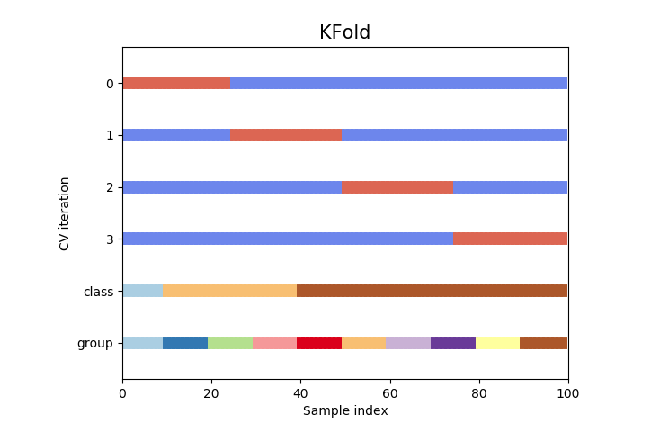
The above procedure reduces variability and hence K-fold cross-validation gives us a more accurate estimate of a model’s performance on out of sample data. Let us now implement 10-fold cross-validation for our model in scikit learn:
In [20]:
# importing cross_val_score function from the model_selection sub-module of scikit learn
from sklearn.model_selection import cross_val_score
# Saving the accuracy scores for a 10 fold cross validation in Accuracy_scores
Accuracy_scores = cross_val_score(knn6, X, y, cv=10, scoring='accuracy')
#Printing all 10 accuracy scores
print(Accuracy_scores)
[1. 0.93333333 1. 1. 0.86666667 0.93333333
 0.93333333 1. 1. 1. ]
In [21]:
# Taking the average of all 10 accuracy scores
print(Accuracy_scores.mean())
0.9666666666666668
This average value of 0.9666 is a better estimate of the accuracy of our model compared to 0.9473 obtained earlier i.e. our initial train-test split had underestimated the predictive power of knn6 model for out of sample data.
Hyperparameter tuning using GridsearchCV in scikit learn
Earlier, we had randomly chosen the value of hyperparameter k of our kNN model to be six and conveniently named our model knn6. We left all other hyperparameters to their default values. However, we do not know if this set of hyperparameters produces the most optimal decision boundary between the three Iris species. So, instead of doing trial-error to find the values of the parameters, a better approach will be to use an algorithm which automatically finds the best set of parameters for a particular model. GridSearchCV is one such algorithm which finds the optimal set of hyperparameter values we are looking for.
GridSearchCV makes use of cross-validation concept (discussed earlier) to find the accuracy for all the possible combinations of hyperparameter values and automatically finds and fits the best one.
Let us consider the example of a kNN algorithm which we have considered thus far. Suppose we want to tune two of the hyperparameters for a kNN model namely:
- n_neighbors (aka k) and
- leaf_size
We can define an object containing potential values for these parameters as follows:
In [18]:
# importing GridSearchCV algorithm from the model_selection sub-module of scikit learn
from sklearn.model_selection import GridSearchCV
#Define an object containing hyperparameter name and potential values as key-value pairs
hyperparameter_values = {'n_neighbors':[1,3,5,7,9,11], 'leaf_size':[20,25,30,35,40]}
Thus, in total there are thirty (6X5) possible combinations for the values of hyperparameters and hence thirty possibilities for the kNN estimator.
Let us implement the GridSearchCV algorithm to find the best one and then fit the data to it:
In [24]:
# Instantiating the GridSearchCV algorithm
gs=GridSearchCV(KNeighborsClassifier(),hyperparameter_values,cv=10)
# fitting the data
gs.results=gs.fit(X,y)
What we did here is akin to conducting a 10-fold cross-validation on each of the thirty possible estimators and saving the best result in the object named 'gs'. We can now access he best estimator, parameter values and accuracy score as follows:
In [37]:
print('Best estimator/model: ',gs.results.best_estimator_)
print('Best parameter combination: ',gs.results.best_params_)
print('Best accuracy score: ',gs.results.best_score_)
Best estimator/model: KNeighborsClassifier(algorithm='auto', leaf_size=20, metric='minkowski',
 metric_params=None, n_jobs=None, n_neighbors=9, p=2,
 weights='uniform')
Best parameter combination: {'leaf_size': 20, 'n_neighbors': 9}
Best accuracy score: 0.9733333333333334
The best estimator is kNN model with k(n_neighbor) value of 9 and leaf_size=20, which produces an accuracy score of 0.9733, a marked improvement from a cross-validated score of 0.966 of the knn6 estimator calculated earlier.
Saving the best model for future use
Now that we have worked hard to build an optimal model, we can save it for future use as a pickle file using joblib library (joblib contains a set of tools providing light-weight pipelining in Python) as follows:
In [40]:
# !pip install joblib (if not installed already)
import joblib
#Save model for future use with a pickle file extension
joblib.dump(gs, 'kNN_optimized.pkl')
#To load it back use
joblib.load('kNN_optimized.pkl')
Out[40]:
GridSearchCV(cv=10, error_score='raise-deprecating',
 estimator=KNeighborsClassifier(algorithm='auto', leaf_size=30,
 metric='minkowski',
 metric_params=None, n_jobs=None,
 n_neighbors=5, p=2,
 weights='uniform'),
 iid='warn', n_jobs=None,
 param_grid={'leaf_size': [20, 25, 30, 35, 40],
 'n_neighbors': [1, 3, 5, 7, 9, 11]},
 pre_dispatch='2*n_jobs', refit=True, return_train_score=False,
 scoring=None, verbose=0)
Conclusion
Thus, we have understood how to install and import the scikit learn library. We also went through all the steps for training and optimizing a classification model using scikit learn. In the next blog we will look at how we can train and fine-tune a regression model in scikit learn.
Happy learning till then!
There are many people who might be new to Python or programming in general or never created any trading strategy. The learning curve could be steep if you are a beginner in both these skills. However, you can build the required skills gradually and practice regularly on the hands-on learning exercises given in our course by enrolling here: Algorithmic Trading for Everyone.
If you want to learn various aspects of Algorithmic trading then check out our Executive Programme in Algorithmic Trading (EPAT®). The course covers training modules like Statistics & Econometrics, Financial Computing & Technology, and Algorithmic & Quantitative Trading. EPAT® is designed to equip you with the right skill sets to be a successful trader. Enroll now!
Disclaimer: All investments and trading in the stock market involve risk. Any decisions to place trades in the financial markets, including trading in stock or options or other financial instruments is a personal decision that should only be made after thorough research, including a personal risk and financial assessment and the engagement of professional assistance to the extent you believe necessary. The trading strategies or related information mentioned in this article is for informational purposes only.
