Portfolio Assets Allocation with Machine Learning

As is often the case, Machine Learning (ML) techniques outperform traditional ones when allocating weights to different assets. The idea of this project "Portfolio Assets Allocation: A practical and scalable framework for Machine Learning Development" is to design a market neutral (long/short) portfolio of assets to be rebalanced periodically choosing different assets during every rebalance and evaluate different portfolio techniques such as:

• Equal Weighted Portfolio (EWP),
• Inverse Volatility Portfolio (IVP),
• Hierarchical Risk Parity (HRP), and
• Hierarchical Equal Risk Contribution (HERC).

This article is the final project submitted by the author as a part of his coursework in the Executive Programme in Algorithmic Trading (EPAT) at QuantInsti. Do check our Projects page and have a look at what our students are building.

About the Author

Raimondo Marino is a professional freelance working as an Artificial intelligence Engineer for Italian Small and Medium Companies. Through AI applications, he comes up with end to end solutions (from Development to Production using cloud services) for different corporate functions within a company: Marketing, HR, Sales, Production, etc.

He is also a passionate quant-trader who believes in the efficacy of combining Machine Learning techniques with Statistics and Probability to design superior trading systems.

He holds a M.Sc. in Electronic Engineering from the University of Naples (Italy), an Executive MBA from SDA Bocconi of Milan (Italy) and a Postgraduate in Machine Learning and Artificial Intelligence from Columbia Business Executive Education (USA).

Acknowledgments

I am deeply grateful to my EPAT mentor Dhiraj Yashwantrao for his outstanding support throughout the entire course and to my project mentor Ishan Shah for his precious and practical advice on how to carry out this project. I was stuck a couple of times and he brilliantly helped me find the right solution.

Recording of the Presentation

Slide deck

Project Abstract

A framework for portfolio allocation for both traditional and Machine learning model based (henceforth referred to as ML) was developed to design and evaluate different portfolio techniques such as:

• Equal Weighted Portfolio (EWP),
• Inverse Volatility Portfolio (IVP),
• Hierarchical Risk Parity (HRP), and
• Hierarchical Equal Risk Contribution (HERC).

As it is often the case, ML techniques outperform traditional ones when allocating weights to different assets therefore providing superior performances and greater risk reduction through better diversification.

The idea was to design a market neutral (long/short) portfolio of assets to be rebalanced periodically choosing different assets during every rebalance.

The criteria used for selecting assets during the rebalance for the long/short portfolio was the Cross-Sectional Momentum trading strategy. Then, using different portfolio techniques, an unlevered and normalized weight allocation was performed on the asset universe.

This process was followed by a vectorized backtest whose objective was to assess the performances of the different techniques.

Lastly, a Monte Carlo simulation was conducted on the best portfolio to properly size the amount of money to be invested during the periodic portfolio rebalancing. Specifically, two metrics were simulated:

• the Terminal Wealth, and
• the Max DrawDown.

Moreover, there was no parameter optimization since HRP and HERC are ML techniques in the realm of Unsupervised Learning field (there are no labels). This way we prevented the risk of overfitting (i.e. learn the noise rather than the true signal).

The signal noise ratio is in fact notoriously low for financial data. Everything was accomplished through python classes that allow for a fast and smooth transition from Development to Production environments.

Another technique used for improving the code efficiency was the use of the multiprocessing python module that allows the use of parallel computing (multiple CPUs) when performing backtesting on thousands of different parameter combinations.

Data gathering and normalization

A demo account was setup with FXCM, one of the few online brokers that offers free access to historical data for almost 60 financial instruments ranging from currency pairs, indices and commodities.

We chose to download daily data for 57 assets starting from 2010 up to the time of writing this document. We also split the data into to train and test sets, perform our analysis on the train set and use the test set only once to validate the results.

Then we calculated the returns for different time periods: 1, 5 and 10 days. We also had to normalize the starting date since instruments had different starting dates.

Another aspect was that we didn’t apply any a priori filtering to the asset universe, mainly because all the assets were derivative CFDs (Contract for Difference).

Liquidity is normally not an issue when buying or selling this type of assets (the hypothesis holds up to a point and if we don’t buy/sell massive quantity of them which is precisely our case).

Phase 1: Feature Engineering Module

The first step for building our framework was adding features. The only limit when adding or inventing features is our imagination and the computational resources available.

We chose to add several technical indicators repeating each of them with different parameters. We made use of Ta-Lib python library and of the following indicators:

We ended up with more than 90 features.

Area of improvement

The framework allows to easily add other features. We are going to implement new ones like fundamental data, date features, sentiment features, trend/seasonality, regime changes ones, different timeframes and so on.

Phase 2: Feature Selection Module:

During this phase the following basic steps were performed:

• Check for feature stationarity: we removed the non-stationary features since all statistical and Machine Learning models require the stationarity of data to perform well.
• Basic filtering: constant, quasi-constant and duplicated features were removed since they do not add any value to ML models.
• Multicollinearity: it is known that collinearity is a big problem for both linear statistical and ML models. We decided to remove at least the linear correlation among the features through an innovative recursive procedure. For this purpose, the standard Pearson correlation index was used.

Area of improvement

Instead of removing the non-stationary features, we plan to use the Fractional Differentiation that combines the benefits of retaining most of the information within the features (instead of discarding them) while at the same time getting the required minimum stationarity for ML models.

Phase 3: Portfolio Optimization and Weights Allocation

This step is divided into two parts:

1. Apply the Cross-Sectional Momentum strategy to all the financial assets on a holding period basis for all possible combination of the following parameters:
a. Lookback period: from 12 to 56 weeks
b. Skip Period: from 1 to 4 weeks
c. Holding Period: from 1 to 4 weeks

Due to high number of combinations (more than 700 heavy computations were required - this is a CPU-bound process) we used the multiprocessing python module to speed up the computation.

It is worth mentioning that the Cross-Sectional Momentum might be found looking at historical data in medium term periods (from 2/3 months to 1 year) so our lookback parameter was chosen starting from 3 months up to 1 year.

Furthermore, it is often true that a short-term reversal effect applies to the most recent data. To handle this phenomenon, we introduced the skip period parameter (from 1 to 4 weeks) to exclude the most recent data from the analysis.

Finally, a third parameter was introduced: the holding period (from 1 to 4 weeks) that is the time during which a portfolio rebalance is performed.

2. For every combination of parameters and for every week, we identified the long/short portfolio to which we applied the different portfolio techniques mentioned earlier after normalizing all the features to account for different ranges in which the features vary.

The results were the weekly normalized weights based on the parameters specified (lookback, skip and holding period).

Area of improvement

First off, we can easily add new portfolio techniques with this framework. Then Instead of applying the Cross-Sectional Momentum that requires:

• going long with the top performers (considering the returns in the upper 10 percentile) and
• going short with the worst performers (in the bottom 10 percentile)

We plan to apply some ML tree models (like gradient boosting, ensemble of learners etc.) to select the long/short assets during the rebalancing. Moreover, the beta of the assets was neglected since we do not have an index representative of our universe to compare our strategies with.

One way to get around this problem could be to build a synthetic portfolio of all the assets considered in the asset universe. This way we could obtain a benchmark to compare the different techniques with.

Lastly when the number of combinations to test is very high (more than 100.000) in addition to multiprocessing (already implemented in our framework) it is advisable to use more sophisticated python frameworks like Optuna, SciKit Optimize, Ray Tune, etc.. to look for the optimal parameters instead of applying the exhaustive Grid Search technique that is not scalable.

Phase 4: Backtesting and Evaluation

We applied the vectorized backtesting to more than 3,000 combinations of parameters and techniques from the previous step and the following table shows the best/worst performers.

Different metrics were calculated:

Best performers

Worst performers

We can see that the best techniques (ranked first by the Sharpe Ratio and then by the Max DD) are the ones that derive from ML namely: HRP and HERC with one exception being the classic Inverse Volatility Portfolio model (IVP).

Another result is that the best performers have a lookback period between 36 weeks and 49 weeks while the worst performers have a shorter lookback period between 13 and 23 weeks.

This is sign of a robust framework where the probabilities of overfitting are very low. However, the best system is not ready to be tradable yet (max SR is 0.5). The framework needs to be improved.

Area of improvement

Instead of using the traditional train/test split that uses only one path, we plan to improve the backtesting using the Combinatorial Purged Cross Validation (CPCV), a brilliant method devised by Lopez Del Prado in his famous book: “Advances in Financial Machine Learning”.

This method overcomes the limitations imposed by traditional train/test split, Cross-Validation and even the Walk Forward analysis by simulating all the possible paths thereby preventing leakage, overfitting and producing more robust statistics on future performances.

Phase 5: Montecarlo Simulation

Point estimates of trading systems performances are just the starting point of a trading systems analysis and should never be relied upon as standalone measures.

We should remember that even a perfectly flawless trading system when put into production with real money is nothing more than a succession of events that happen one after the other with a certain probability and that the entire sequence of trades can only be considered one realization among hundreds of thousands of possible paths.

The real path can hopefully produce better results but most often it will produce worse results than the point estimates we calculated in our analysis.

Therefore, it is essential to estimate the variability of the point estimates and change our position size accordingly (in our simulation we didn’t use any leverage since the best system is not yet tradable without further improvements).

Below we see the graphs produced for the best portfolio techniques and the relative parameters by generating 3.000 paths for the Terminal Wealth and the max Drawdown that, together with the Sharpe Ratio, are the most common measures we are interested in when evaluating trading systems performances.

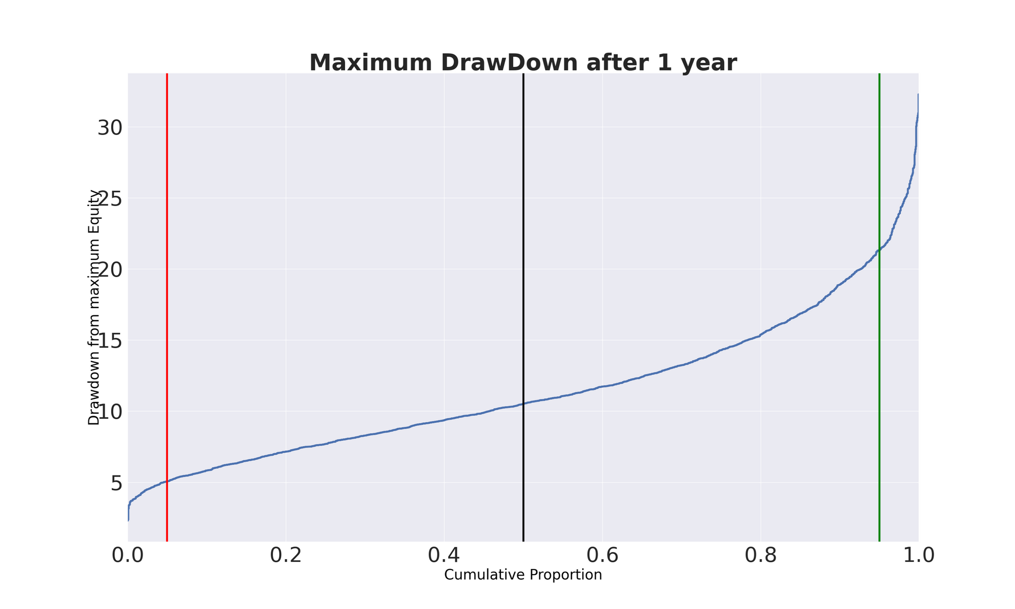
From this graph we can conclude that our TW after 1 year varies between 85% and 131% of the starting capital in 90% of the cases, while the Max DrawDown ranges roughly between 5% and 21% with 90% of probability.

Of course, there is always the case of a Black Swan that lives in the tail of the distribution. We need to be comfortable with uncertainty when evaluating the future. Here you can see in action the power of Montecarlo simulation– an invaluable method for quantitative traders.

Area of improvement

Montecarlo simulation is a parametric method based on the hypothesis that returns are normally distributed which is almost never the case (returns are better modelled with the Cauchy distribution which is more difficult to model and estimate).

There are many variations to the plain vanilla Montecarlo simulation we applied in this project, to name a few:

• Geometric Brownian Motion, and
• Multivariate Gaussian distribution.

They are only slightly more precise than plain Montecarlo but far more complicated to implement.

Another way we could simulate the future is by using the non-parametric Bootstrapping methods that are distribution-free and, differently from Montecarlo, do not rely on any assumption about the underlying data generation process.

We are currently planning to implement the Bootstrapping procedure since this method relies on different assumptions than the plain vanilla Montecarlo. Then we could compare the two procedures so that we may form a better opinion of future performances of our trading system.

Next Steps

Apart from the improvements depicted above for each module, there will be a final module on money management and position sizing. Use of leverage, transactions, slippage and other costs will be also part of this module that will help decide on capital allocation and position sizing.

Lastly, we will put the overall framework into production using AWS Cloud Services. There are many solutions available to choose from.

Bibliography/Resources

1. Book: "Advances in financial Machine Learning"  by Lopez del Prado 2018
2. Book: "High Performance Python" Gorelick and Ozsvald 2014
3. Free dowloadable guide: https://hudsonthames.org/modern-guide-to-portfolio-optimization/
4. Python library on portfolio optimization: Riskfolio lib https://riskfolio-lib.readthedocs.io/en/latest/

Conclusion

The main idea for this project was to develop a robust framework that could be useful and scalable when testing different portfolio techniques for both traditional and ML based.

Due to the enormous quantity of data to process (many assets with many features and different timeframes even with a medium-low frequency trading strategy) we need a way to leverage the multi-CPU technology available in modern PCs.

This can be accomplished using the python multiprocessing module and some python packages. They are typically used in the case of Neural Networks which generally require the optimization of millions of parameters.

In our case we are considering hundreds of thousands of simulations. If not properly addressed, processing lots of data, like in the case of portfolios asset allocation, can be quite cumbersome if not impossible.

Applying the framework to FXCM data, we showed the superiority of ML portfolio allocation models like Hierarchical Risk Parity and Hierarchical Equal Risk Contribution over traditional techniques.

Moreover, it was shown the robustness of the framework since the range of the lookback period for the best and worst performers was very low. We won’t stop here of course!

We will keep improving the framework as depicted above until we reach the stage of producing a tradable system.

If you want to learn various aspects of Algorithmic trading then check out this algo trading course which covers training modules like Statistics & Econometrics, Financial Computing & Technology, and Algorithmic & Quantitative Trading. EPAT equips you with the required skill sets to build a promising career in algorithmic trading. Enroll now!

File in the download

• Phase 4 - best performers output data (MS Excel file)
• Phase 4 - worst performers output data (MS Excel file)

Login to Download

Note: The code and the relevant data files are withheld at the author's request. Kindly reach out to us at sales@quantinsti.com in case of any queries.

Disclaimer: The information in this project is true and complete to the best of our Student’s knowledge. All recommendations are made without guarantee on the part of the student or QuantInsti^®. The student and QuantInsti^® disclaim any liability in connection with the use of this information. All content provided in this project is for informational purposes only and we do not guarantee that by using the guidance you will derive a certain profit.