Introduction to Support Vector Machines

By Varun Divakar

Support Vector Machines were widely used a decade back, but now they have fallen out of favour. The below data from google trends can establish this more clearly.

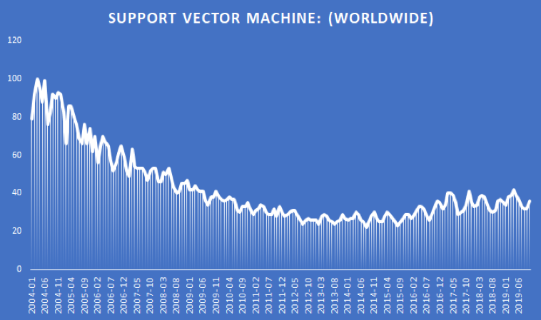
(Source: Google Trends)

Why did this happen?

As more and more advanced models were developed, support vector machines fell out of favour. It takes a lot of time to train a non-linear kernel, say RBF (Radial Basis Function), of a support vector machine. But they have been found to be very effective in text classification problems. Support Vector Machines (SVMs) are also good at solving non-linear problems with a small dataset. This is precisely the reason why I prefer SVMs in trading. 

Support Vector Machines in trading 

When it comes to trading, if you are using daily frequency data, then it is very likely that your data set is extremely limited, probably a few thousand data points. Let us say that you have created a trading strategy using a decision tree to extract a high probability rule from the past data. Now you want to understand how this rule would behave on unseen or test data. Creating an SVC to predict when the rule would be a success or failure would help you eliminate the bad trades. Before you try out the SVMs, first let us understand how they work.

Thus, in this article, we will cover the following topics:

• Support Vector Machines
• Understanding Support Vector Machines with an example
• Mathematics of Support Vector Machines
• Soft Margin Classifier
• Non-linear Model
• Trading using Support Vector Machines in Python

Support Vector Machines

A Support Vector Machine is an approach, usually used for performing classification tasks, that uses a separating hyperplane in multidimensional space to perform a given task. Technically speaking, in a p dimensional space, a hyperplane is a flat subspace with p-1 dimensions. For example, In two-dimensions, a hyperplane is a flat one-dimensional subspace or a line. In three dimensions, a hyperplane is a flat two-dimensional subspace that is, a plane. 

If the dimensionality is greater than 3, it can be hard to visualize a hyperplane, but the notion of a p-1 dimensional space still applies. 

Understanding Support Vector Machines with an example

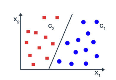
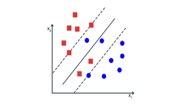
Now that you have a basic understanding of hyperplane, let us understand the intuition behind the Support Vector Machine. Consider a data set of two different classes, shown in blue and red.

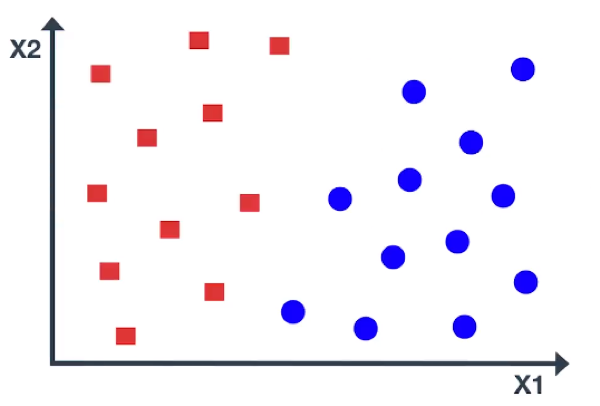
The data is linearly separable, and there exist multiple separating lines, which are shown in black. All these lines offer a solution, but only one line is optimal and can separate the classes accurately.

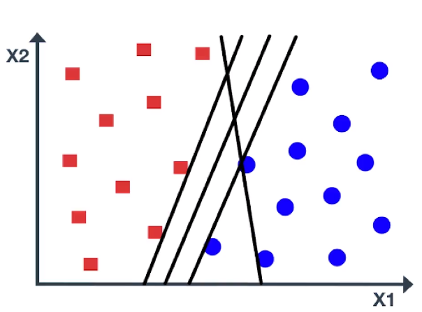
For example, If the line is very close to the data points, even a small noise would lead to misclassification. Here is another line that separates the classes, but doesn’t look like a very natural one. So, the question is which is the best line? 

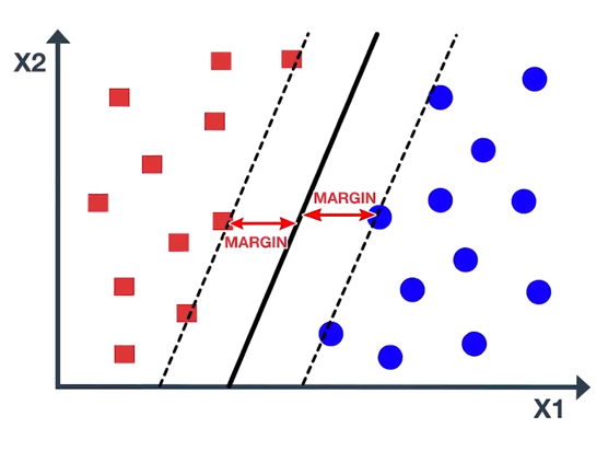
Support Vector Machine chooses an optimal line which maximizes the distance to the nearest points in either class. This distance is called the margin. As you can see in the figure, the margin is the distance from the solid line to either of the dashed lines.

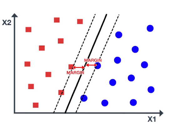
Our aim is to maximize the margin as large as possible in order to get an optimal line. So, the Support Vector Machine is sometimes called Maximum Margin Classifier. In the figure, there are some blue and red data points on the dashed lines. These points are known as support vectors. It is important to note that the maximum margin line or decision boundary depends only on the support vectors, but not on other data points.

As you can see in the figure, moving the support vectors, also moves the maximum margin line, while moving the other points has no effect. Maximum margin line is only useful when the data is linearly separable, Or in other words, data can be separated by a straight line. In the figure, the data points belong to two classes and are not necessarily separable by a maximum margin line. In fact, if a separating line does exist, it is not optimal, as it misclassifies and has a small margin. So, what approach should we implement when the data is non-linear?

In that case, we consider enlarging the feature space, such as quadratic, cubic, or even higher-order polynomial, to address this non-linearity. We can enlarge the feature space in a specific way, by using a function which is known as ‘Kernel’. Let us understand kernel is and some of the mathematics behind support vector machines.

Mathematics of support vector machines

The key points for you to understand about support vector machines are:

1. Support vector machines find a hyperplane (that classifies data) by maximizing the distance between the plane and nearest input data points (called support vectors).
2. This is done by minimizing the weight vector ‘w’ which is used to define the hyperplane.
3. Step 2 relies on optimization theory and certain assumptions (which are detailed out below). 

Maximising the distance between hyperplane and support vectors

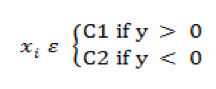
For simplicity, consider the linearly separable data points that belong to either class C₁ or class C₂ with no misclassification for any data points.

For an unknown input data x, we define a linear discriminate function. 

y = f(x) = w. x + b 

where w is the weight vector which is perpendicular to the hyperplane. 

b is the bias term

...(1)

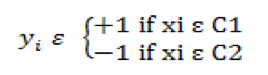
Let all input points be represented by x₁, …, x_p and their corresponding class be represented by y₁, …, y_p. So, if x_i belongs to class c₁, then corresponding y_i is equal to +1 and if x_ii belongs to class c₂, then corresponding y_i is equal to -1.

... (2)

Earlier, we assume that data points belonging to two classes are linearly separable. Then it is possible to select two hyperplanes in a way that there are no points between them and then try to maximize the distance between the two hyperplanes. Such type of Support Vector Machine is known as Hard Margin SVM.

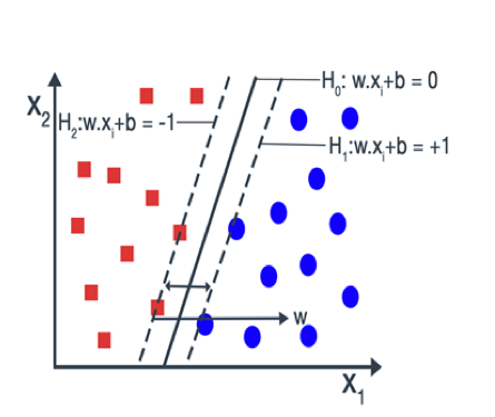
The two hyperplanes can be best represented by the equation

H1 : w.x_i + b = -1 ... (3)

H2 : w.x_i + b = 1 ... (4)

Suppose x₁ and x₂ be the two closest points on each side of the hyperplane. Then, the equations for the hyperplanes H1 and H2 become:

w.x₁ + b = -1 ... (5)

w.x₂ + b = +1 ... (6)

By differencing the equation (5) and equation (6) we get, 

w (x₁ - x₂ ) = 2 ... (7)

Dividing both sides of the equation (7) by the magnitude of the ‘w’ we get,

w (x₁ - x₂ ) / ||w|| = 2 / ||w|| ... (8)

As we know, when we divide a vector with its magnitude, we get a unit vector. And the magnitude of the unit vector is 1. So, our equation becomes:

(x₁ - x₂ ) = 2 / ||w|| ... (9)

(x₁ - x₂ ) is the distance between the two hyperplanes. So, the distance which we are going to maximize is 2 / ||w||. To maximize 2 / ||w|| is to minimize ||w|| and in order to prevent the data points falling into the margin, we add the following constraints.

Minimize 2 / ||w|| ... (10)

Multiplying both equations by their corresponding y_i they are transformed into just one equation

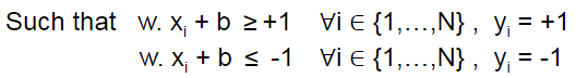
y_i (w. x_i + b)≥1 &nbsp ∀i ∈ {1,…,N}

The above optimization problem is difficult to solve but it is possible to alter the equation substituting 2/ ||w|| by ½ ||w||2 without changing the solution. The problem now belongs to the quadratic programming (QP) optimization that is easier to be computed.

Minimize ½ ||w||² ... (11)

Such that y_i (w. x_i + b)≥1, &nbsp ∀i ∈ {1,…,N}

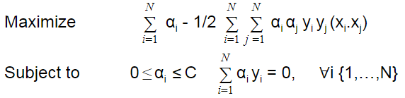
This is the quadratic optimization problem or primal form. This primal problem can be converted into another optimization problem i.e. dual problem with the help of Lagrangian multiplier. 

Dual optimization equation with lagrangian multiplier is given below:

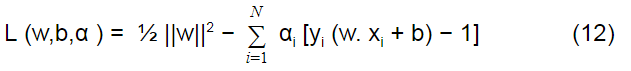
Subject to α_i>=0 ∀i ∈ {1,…,N}

where αi is a Lagrangian multiplier 

By multiplying the components in the bracket of the equation (12):

Setting the derivative of L w.r.t w and b individually to 0:

∂L/∂b = - Σ αi y_i = 0

⇒ Σαi y_i = 0 ... (13)

∂L/∂w = w - Σ αi y_i x_i = 0

⇒ w = Σ αi y_i x_ii ... (14)

Substituting the values of equation (13) and (14) in L we get,

L = ½ Σ Σαi αj y_i y_j( x_i.x_j) - ΣΣαi αj y_i y_j(x_i.x_j) + Σ αi

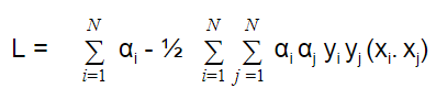
Here, Our aim is to maximize the dual optimization problem for different values of lagrangian multiplier i.e. α.

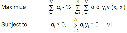
One Important thing to note is that if the Lagrangian multiplier i.e αi = 0 then the data points are not support vectors. So, only for αi > 0, x_i are support vectors (SV).

Soft Margin Classifier

The above optimization problem is only useful when the data points are classified correctly meaning there are no points between the margin. Sometimes high noise in the data causes overlap of the classes as shown in the figure.

In such cases, we can do the classification task by using Soft Margin SVM.

A soft-margin SVM provides freedom to the model to misclassify some data points by minimizing the number of such samples. Soft-margin SVM allows for the possibility of violating the constraints

y_i (w.x_i + b)≥1 ∀i ∈ {1,…,N}

by introducing slack variable ξi

y_i (w.x_i + b)≥1 - ξi ξi ≥0 ∀i ∈ {1,…,N}

Now, our goal is to maximize the margin by keeping the ξi as small as possible.

Our Primal or quadratic optimization problem after introducing slack variable:

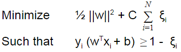
Here, C is a regularization parameter (trade-off between classification and error). Transforming to the lagrangian dual problem we obtain:

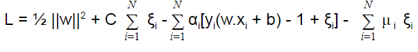
Here, μ_i are the new lagrangian multipliers.

After taking partial derivative of L w.r.t w and b separately to 0. Our dual optimization problem becomes:

This is very similar to the hard margin case, except the value of α_i lies between 0 and C.

Non-linear Model

What we learnt till now is only applicable when the data is linearly separable. When the data is non-separable these optimization problems are not feasible. Such a problem can be solved by enlarging the feature space through a function known as the kernel.

Mathematically, a kernel is some function that corresponds to an inner product in some expanded feature space. If every data point is mapped into high-dimensional space via some transformation Φ: x → φ(x), then the kernel function is defined as: 

K(x_i ,xj )= φ(x_i ). φ(xj)

We can modify our optimization problem by introducing kernel function as:

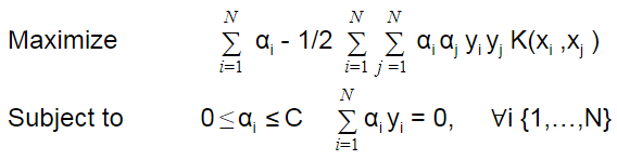
(Source: Wikipedia)

Thus, we have seen the intricacies of the Support Vector Machines along with its applications as a non-linear model. We have also understood what it means by a Soft Margin Classifier and how it overcomes the optimisation problem in the support vector machines model. 

In the next section, I will show you how to implement a machine learning based trading strategy using the regime predictions made in an earlier blog.

There is one thing that you should keep in mind before you read this section though: The algorithm is just for demonstration and should not be used for real trading without proper optimization.

Trading using Support Vector Machines in Python

Let me begin by explaining the agenda here:

1. Create an unsupervised ML ( machine learning) algorithm to predict the regimes.
2. Plot these regimes to visualize them.
3. Train a Support Vector Classifier algorithm with the regime as one of the features.
4. Use this Support Vector Classifier algorithm to predict the current day’s trend at the Opening of the market.
5. Visualize the performance of this strategy on the test data.
6. Downloadable code for your benefit

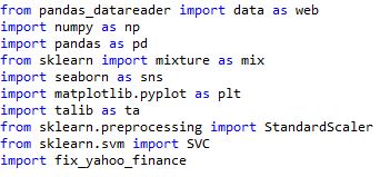
Import the Libraries and the Data:

First, I imported the necessary libraries. Please note that I have imported fixyahoofinance package, so I am able to pull data from yahoo. If you do not have this package, I suggest you install it first or change your data source to google.

Next, I pulled the data of the same quote, ‘SPY’, which we used in the previous blog and saved it as a dataframe df. I chose the time period for this data to be from the year 2000.

After this, I created indicators that can be used as features for training the algorithm.

But, before doing that I decided on the look back time period for these indicators. I chose a look back period of 10 days. You may try any other number that suits you. I chose 10 to check for the past 2 weeks of trading data and to avoid noise inherent in smaller look back periods.

Apart from the look back period let us also decide the test train split of the data. I prefer to give 80% data for training and remaining 20% data for testing. You can change this as per your need.

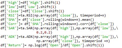
Next, I shifted the High, Low and Close columns by 1, to access only the past data. After this, I created various technical indicators such as, RSI, SMA, ADX, Correlation, Parabolic SAR, and the Return of the past 1- day on an Open to Open basis.

Next, I printed the data frame.

And it looked like this:

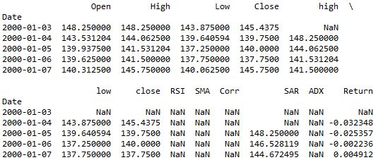
As you can see, there are many NaN values. We need to either impute them or drop them. If you are new to the machine learning and want to learn about the imputer function, read this. I dropped the NaN values in this algorithm.

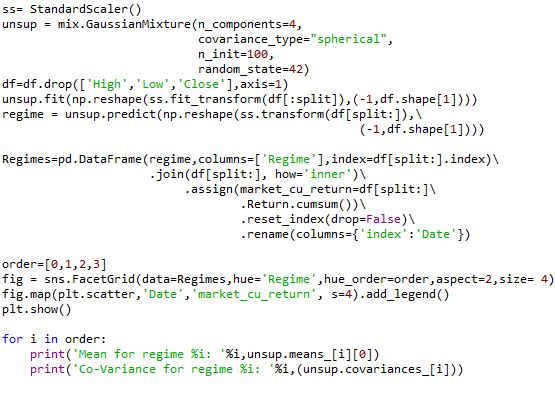
In the next part of the code, I instantiated a StandardScaler function and created an unsupervised learning algorithm to make the regime prediction. I have discussed this in my previous blog, so I will not be going into these details again. Explore the 'Unsupervised Learning Course' from Quantra.

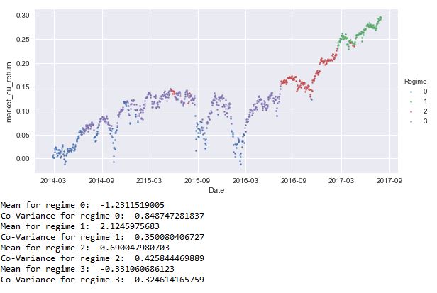
Towards the end of the last blog, I printed the Mean and Covariance values for all the regimes and plotted the regimes. The new output with indicators as feature set would look like this:

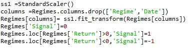
Next, I scaled the Regimes data frame, excluding the Date and Regimes columns, created in the earlier piece of code and saved it back in the same columns. By doing so, I will not be losing any features but the data will be scaled and ready for training the support vector classifier algorithm. Next, I created a signal column which would act as the prediction values. The algorithm would train on the features’ set to predict this signal.

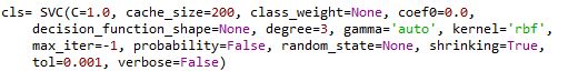
Next, I instantiated a support vector classifier. For this, I used the same SVC  model used in the example by sklearn. I have not optimized this support vector classifier for best hyper parameters. In the machine learning course on Quantra®, we have extensively discussed how to use hyper parameters and optimize the algorithm to predict the daily Highs and Lows, in turn the volatility of the day.

Coming back to the blog, the code for support vector classifier is as below:

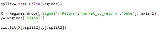
Next, I split the test data of the unsupervised regime algorithm into train and test data. We use this new train data to train our support vector classifier algorithm. To create the train data I dropped the columns that are not a part of the feature set:

'Signal','Return','marketcureturn','Date'

Then I fit the X and y data sets to the algorithm to train it on.

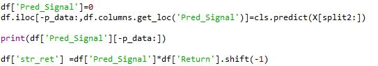
Next, I calculated the test set size and indexed the predictions accordingly to the data frame df.

The reason for doing this is that the original return values of ‘SPY’ are stored in df, while those in Regimes is scaled hence, won’t be useful for taking a cumulative sum to check for the performance.

Next, I saved the predictions made by the SVC in a column named Pred_Signal.

Then, based on these signals I calculated the returns of the strategy by multiplying signal at the beginning of the day with the return at the opening ( because our returns are from open to open) of the next day.

Finally, I calculated the cumulative strategy returns and the cumulative market returns and saved them in df. Then, I calculated the sharpe ratio to measure the performance. To get a clear understanding of this metric I plotted the performance to measure it.

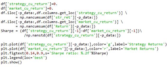
The final result looks like this.

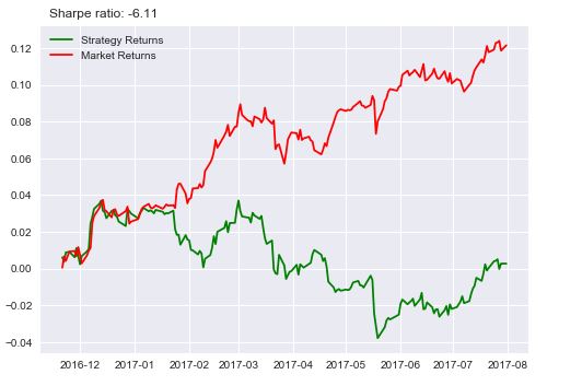
After so much of code and effort, if the end result looks like this, then someone with no machine learning back ground would say that it is not worth it. I would agree for now. But, look at this line of code:

I just changed the data from SPY to IBM. Then the result looks like this:

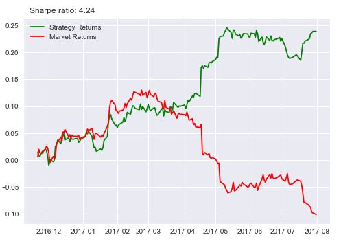
I know what you are thinking: I am just fitting the data to get the results. Which is not entirely wrong. I will show you another stock then you decide.

I changed the stock to Freeport-McMoRan Inc and the result looks like this:

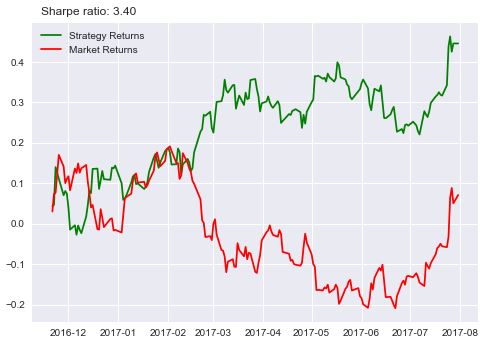
You can further change it to GE or something else and check for yourself. This strategy works on some stocks but doesn’t work on others, which is the case with most quant strategies. There are a few reasons why the algorithm did work consistently and I will list some of them here.

1. No autocorrelation of returns
2. No Support Vector hyper parameter optimization
3. No error propagation
4. No feature selection

We have not checked for autocorrelation of the returns, which would have increased the predictability of the algorithm. Try that on your own by shifting the returns column by 1 and passing it as feature set. The result would look like this:

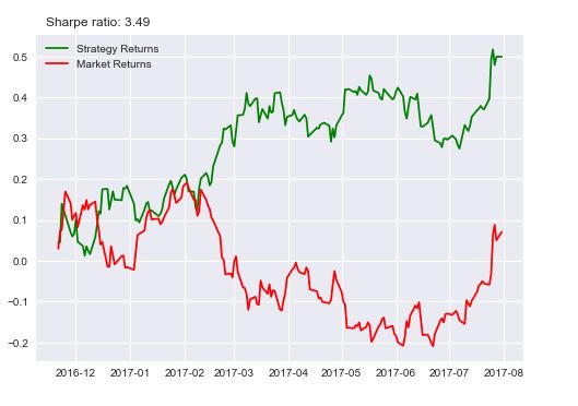
Although the improvement from 3.4 to 3.49 is not much, it is still a good feature to have.

Please note that the code will best run with Python 2.7

Update

We have noticed that some users are facing challenges while downloading the market data from Yahoo and Google Finance platforms. In case you are looking for an alternative source for market data, you can use Quandl for the same. 

Conclusion

Thus, not only have we seen the mathematics behind the Support Vector Machine, but we have also understood how to build a trading strategy using SVM in Python.

If you want to learn how to use Support vector machines on financial markets data and create your own prediction algorithm, you can enroll for the Trading with Machine Learning: Classification and SVM course which covers classification algorithms, performance measures in machine learning, hyper-parameters and building of supervised classifiers.

If you want to learn various aspects of Algorithmic trading then check out our Executive Programme in Algorithmic Trading (EPAT®). The course covers training modules like Statistics & Econometrics, Financial Computing & Technology, and Algorithmic & Quantitative Trading. EPAT® is designed to equip you with the right skill sets to be a successful trader. Enroll now!

Disclaimer: All data and information provided in this article are for informational purposes only. QuantInsti® makes no representations as to accuracy, completeness, currentness, suitability, or validity of any information in this article and will not be liable for any errors, omissions, or delays in this information or any losses, injuries, or damages arising from its display or use. All information is provided on an as-is basis.

Download Data Files

• Python_3

Login to Download