
By Vivek Krishnamoorthy and Udisha Alok
In this blog, we take a critical look at the assumptions of a linear regression model, how to detect and fix them, and how much water they hold in the real world. We will check some of these assumptions and tests in Python, which will provide a blueprint for other cases using well-known libraries. We will also examine its shortcomings and how its assumptions limit its use.
In the first blog of this series, we deconstructed the linear regression model, its various aliases and types. In the second installment, we looked at the application of linear regression on market data in Python and R.
Our coverage proceeds on the following lines:
- What is Linear Regression?
- Assumptions of linear regression
○ Linear relationship
○ No Multicollinearity
○ No Autocorrelation of the error terms
○ Homoskedasticity of the error terms
○ Zero conditional mean of the error terms
○ Gaussian distribution of the error terms (optional) - Limitations of linear regression
○ Simplistic in some cases
○ Sensitivity to outliers
○ Prone to underfitting
○ Overfitting of complex models - References
What is Linear Regression?
Linear regression models the linear relationship between a response (or dependent) variable (Y) and one or more explanatory (independent) variables (X).
We can express it in the form of the following equation:
\(Y_{i} = \beta _{0}+ \beta_{1}X_{i}+\epsilon _{i}\)In the case of a single explanatory variable, it is called simple linear regression, and if there is more than one explanatory variable, it is multiple linear regression.
In regression analysis, we aim to draw inferences about the population at large by finding the relationships between the dependent and independent variables for the sample. Usually, the OLS (Ordinary Least Squares) method is used to estimate the regression coefficients. OLS finds the best coefficients by minimizing the sum of the squares of the errors.
Top posts on Machine Learning
4 min read
Gauss-Markov theorem
The Gauss-Markov theorem states that under certain conditions, the Ordinary Least Squares (OLS) estimators are the Best Linear Unbiased Estimators (BLUE). This means that when those conditions are met in the dataset, the variance of the OLS model is the smallest out of all the estimators that are linear and unbiased.
Let’s examine the terms ‘linear’ and ‘unbiased’.
- Linear - Linear estimators imply that they have a linear relationship with the dependent variable. This makes them easier to understand and implement.
- Unbiased - Unbiased estimators imply that when applying a model repeatedly, on average, the estimators will attain their true value.
We now look at the “under certain conditions” (i.e. the assumptions) mentioned earlier that form the core of the Gauss-Markov theorem.
Assumptions of Linear Regression
We can divide the basic assumptions of linear regression into two categories based on whether the assumptions are about the explanatory variables (i.e. features) or the residuals.
Assumptions about the explanatory variables (features):
- Linearity
- No multicollinearity
Assumptions about the error terms (residuals):
- Homoskedasticity
- No autocorrelation
- Zero conditional mean
- Gaussian distribution (optional)
Linearity
The basic assumption of the linear regression model, as the name suggests, is that of a linear relationship between the dependent and independent variables. Here the linearity is only with respect to the parameters. Oddly enough, there’s no such restriction on the degree or form of the explanatory variables themselves.
So both the following equations represent linear regression:
\(Y_{i} = \beta _{0}+ \beta_{1}X_{i}+\epsilon _{i}\qquad\qquad - (1)\)Here, the model is linear in parameters as well as linear in the explanatory variable(s).
\(Y_{i} = \beta _{0}+ \beta_{1}X_{i}^{2}+\epsilon _{i}\qquad\qquad- (2)\)This model is linear in parameters and non-linear in the explanatory variable(s).
The explanatory variables can be exponentiated, quadratic, cubic, etc. and it can still be framed as a linear regression problem.
The following equation is NOT linear regression:
\(Y_{i} = \beta _{0}+ \beta_{1}^{2}X_{i}+\epsilon _{i}\qquad\qquad- (3)\)Linear regression minimizes the error (mean-squared error) to estimate the unknown betas by solving a set of linear equations.
What is machine learning classification?
18 min read
When betas take non-linear forms, things get harder and we cannot use the methods we’d mentioned (but not derived!) earlier. Hence, we cannot use linear regression in the case of equation 3. Hence, the linearity (of parameters) assumption is important.
How to detect linearity?
A residual plot helps us identify poor or incorrect curve fitting between the data and the regression model. It is probably the simplest way to check for linearity or lack thereof. A nice even spread is indicative of linearity.
How to fix linearity?
The tricky part now is to get the functional form of the equation right.
- We can try reframing it by applying a non-linear transformation on the independent and/or the dependent term(s). We can transform messy data by normalizing them, taking logs of the original values, etc. This would make the data linear.
- We can also try adding another independent variable to the equation (like \(X^{2}\)).
No Multicollinearity
Another assumption is that the independent variables are not correlated with each other. If there is a linear relationship between one or more explanatory variables, it adds to the complexity of the model without being able to delineate the impact of each explanatory variable on the response variable.
If we were to model the salaries of a group of professionals based on their ages and years of experience.
\(salary_{i} = \beta _{0}+ \beta_{1}(years\; of\; experience)_{i}+\beta_{2}(age\; in\; years)_{i}+ \epsilon _{i}\)Linear regression studies the effect of each of the independent variables (X) on the dependent variable (Y). But when the independent variables are correlated, as in this case, it is difficult to isolate the impact of a single factor on the dependent variable. If you increase the years of experience, the age also will increase.
So did the salary increase due to the experience or the age?
This will affect the accuracy of the coefficients and also the standard errors.
How to detect multicollinearity?
- Check the correlation among the independent variables.
- Variance Inflation Factor
Top posts on Machine Learning
4 min read
How to fix multicollinearity?
One way to deal with multicollinearity among the independent variables is to do dimensionality reduction using techniques like PCA to create uncorrelated features with the maximum variance.
No autocorrelation of the error terms
The residuals in the linear regression model are assumed to be independently and identically distributed (i.i.d.). This implies that each error term is independent and unrelated to the other error terms.
So, knowing one error term tells us nothing about the other(s). Also, all errors have the same distribution, the normal distribution (with zero mean and finite variance).
The error term at a particular point in time should have no correlation with any of the past values. This makes the error terms equivalent to random noise that cannot be predicted.
In the case of correlation between the residuals, the model’s accuracy is affected. Autocorrelation or serial correlation is a problem specific to regression involving time-series data. You can read more about Autocorrelation and Autocovariance.
When working with time-series data, when the value at a particular time t is dependent on its value at a time (\(t-1\)), there is a chance of correlation between the residuals after the model fitting step. If you know the value of a residual at a given time, you have a reasonably good idea about where the next residual will be.
No autocorrelation is a key requirement for the OLS to be an efficient model (as per the Gauss Markov theorem). When this assumption is violated, although the model is still unbiased, its efficiency will be impacted.
The standard errors would increase, and the goodness of fit may be exaggerated. The significant regression coefficients may appear to be statistically significant when they are not.
Top posts on Machine Learning
4 min read

How to detect autocorrelation?
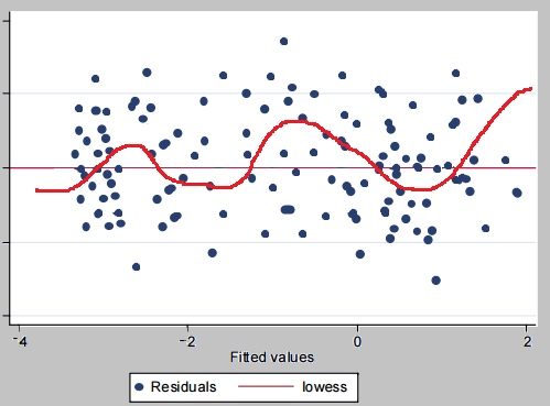
- A snake-like wavy pattern showing sort-of clustering of the residuals in the residual plot indicates autocorrelation of the error terms.
- Durbin-Watson test
How to fix autocorrelation?
- Check for any other parameters influencing the dependent variable and include them in the linear regression model. After including this new \(X\) term, we can check if the residual plot evens out.
- Cochrane-Orchutt procedure
- AR(1) method
What is machine learning classification?
18 min read
Homoskedasticity of the error terms
The term homoskedasticity derives from the Greek words ‘homos’ meaning ‘same’, and ‘skedastikos’, which means ‘scattering’ or ‘dispersion’. Homoskedasticity, therefore, means ‘having the same scatter/variance.’
An important assumption of linear regression is that the error terms have the same variance across all observations. Unequal variance in the error terms is called heteroskedasticity and may be caused due to many reasons like the presence of outliers, or an incorrectly specified model.
The below model tries to estimate the amount an individual gives to charity based on her earnings.
\(charity\;amount_{i} = \beta _{0}+ \beta_{1}(earnings)_{i}+ \epsilon _{i}\)A person having a low income would likely spend less on charity, as she may struggle to meet her own daily expenses. A person in the medium income group may put aside, say, 10% of her income for charity purposes.
What about a person who earns huge amounts of money?
Will the amount of money they contribute to charity also increase proportionally?
You would probably say - it depends on the person’s disposition. This is a typical case of heteroskedasticity.
If we run the regression with heteroskedasticity present, the standard errors would be large and the model would have unreliable predictions.

How to detect homoskedasticity?
- The residual plot can give a good idea of the variance of the residuals. Homoskedastic residuals show no pattern, whereas heteroskedastic residuals show a systematic increasing or decreasing variation (see below for a visual illustration).
Top posts on Machine Learning
4 min read

The Null hypothesis is that the variance in the two sub-samples is the same. The alternative hypothesis can be increasing, i.e. the variance in the second sample is larger than in the first, or decreasing or two-sided. (Source)
This tests the hypothesis that the residual variance does not depend on the variables in \(X\) in the model.
White’s Lagrange Multiplier Test for Heteroskedasticity is more generalized than the Breusch-Pagan test and uses the polynomial and interaction terms of regressors along with them.
How to fix it?
- As discussed earlier, one way to deal with heteroskedasticity is to transform the equation. Taking a log of the dependent variable usually gets rid of the heteroskedasticity.
- Using White’s errors (also known as Robust errors) that correct the standard errors in the OLS for heteroskedasticity. This can be implemented easily using the statsmodels.regression.linear_model.OLSResults.get_robustcov_results. You can read more about it here.
- Use the weighted least squares model, which is an efficient variation of OLS to deal with heteroskedasticity.

What is machine learning classification?
18 min read
Zero conditional mean of the error terms
An important assumption of the classic linear regression model is that the error terms have a conditional mean of zero.
For the following relationship:
\(Y_{i} = \beta _{0}+ X_{i}+ \epsilon _{i} \qquad(where\; i= 1, 2, 3, ...n)\)This assumption can be expressed in the form of the following equation:
\(E(i | Xi) = 0\)This equation means that for any values of the explanatory variables \(X_{1},X_{2},X_{3},...,X_{n}\), the average of the error (which includes the unobserved factors) is zero. So whatever values we select for \(X\), the error term remains completely random. Hence, we cannot get any information about the error term from \(X\).
An exogenous variable is one that is not affected by the other variables in the system. On the contrary, \(X_{i}\) will be endogenous when the \(cov(X_{i}, i) ≠ 0\).
Suppose we wish to estimate the probability of a person contracting COVID-19 based on the time she spends outside her home.
\(probability\;of\;contracting\;infection_{i}=\beta _{0}+ \beta _{1}(time\;spent\;outside\;home)_{i}+\epsilon _{i}\)Now the probability of contracting COVID-19 may also depend on other factors like her profession, daily income, etc. which may be correlated to the time she spends outside home.
We can assume that the time spent outside home is affected by daily income, as a daily wage worker or a homeless person would probably spend more time outdoors.
So, if you regress the probability of contracting infection on the time spent outside home, the estimator for the time spent outside home absorbs the effect of daily income and you get an overly optimistic estimate of the effect of time spent outside home.
This is to say, the effect of time spent outside home on the probability of contracting the infection is (upward) biased because time spent outside home is not exogenous to the probability of getting infected.
Such a model can be used for prediction but not for inferring causation.
What is machine learning classification?
18 min read
Gaussian distribution of the error terms (optional)
Strictly speaking, the classic linear regression model does not require the errors to be normally distributed. Nevertheless, if we impose the normality constraint too, let us see what this means.
The residual (\(\epsilon\)) is the variation in the value of the dependent variable \(Y\), which is not explained by the independent variables. So linear regression assumes that the variability in \(Y\), which is unexplained by \(X\), is normally distributed.
If this assumption is violated, it is not a big problem, especially if we have a large number of observations. This is because the central limit theorem will apply if we have a large number of observations, implying that the sampling distribution will resemble normality irrespective of the parent distribution for large sample sizes.
However, if the number of observations is small and the normality assumption is violated, the standard errors in your model’s output will be unreliable.

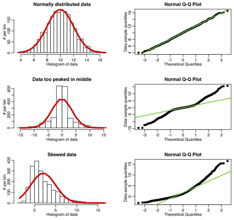
How to detect normality?
- In the residual plot, most points should be centered around zero and should get sparse as we move further away from the best-fit line. The residual means should be zero.
- Q-Q plot
- Anderson-Darling Test
- Shapiro-Wilk Test
- Ryan-Joiner Test
- Kolmogorov-Smirnov Test
How to fix normality?
- The first thing to check is whether we have any outliers. As mentioned earlier, the linear regression model uses the ‘least squares’ to come up with the best fit. So any outliers will severely impact the residuals.
- Add more observations, if possible.
- We can try modifying the functional form of the regression equation by applying nonlinear transformations, as mentioned above.
How to detect omitted variable bias?
There is no straightforward way to check for omitted variable bias. Intuition is probably the best way to go. However, do check the correlation among the independent variables.
How to fix omitted variable bias?
- Using instrumental variables.
What is machine learning classification?
18 min read
Limitations of linear regression
Linear regression is one of the most popular models. When we know that the dependent and independent variables have a linear relationship, this is the best option due to its simplicity and ease of interpretation. However, it has some limitations, which are mentioned below:
Simplistic in some cases
The linear regression model is great for data that has a linear relationship between the dependent and independent variables when the underlying conditions are met. However, that is not always the case. For a lot of real-world applications, especially when dealing with time-series data, it does not fit the bill.
For non-linear relationships (when you see a curve in your residual plot), using logistic regression would be a better option.
An underlying assumption of the linear regression model for time-series data is that the underlying series is stationary. However, this does not hold true for most economic series in their original form are non-stationary.
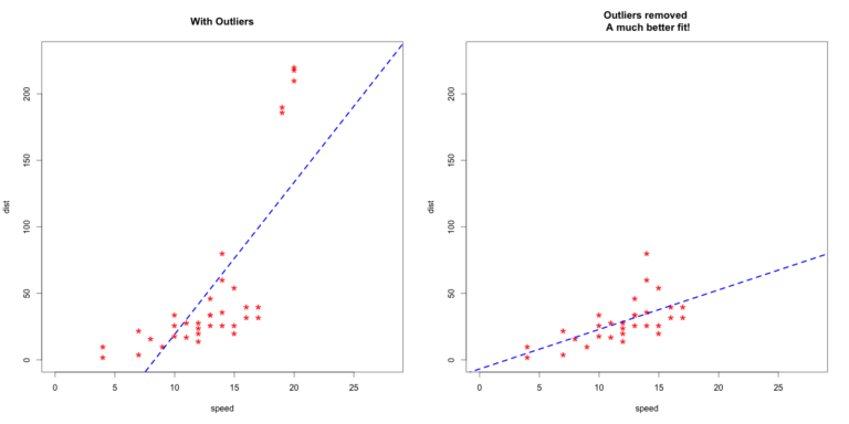
Sensitivity to outliers
As mentioned earlier, the linear regression model uses the OLS model to estimate the coefficients. This model finds the best fit line by minimising the squared sum of errors. So any observation that is away from the major cluster of points will have a squared impact. Consequently, outliers can have an outsize impact on the output of the model.

Top posts on Machine Learning
4 min read
Prone to underfitting
Underfitting occurs when a model cannot adequately capture the underlying structure of the data. Due to the various assumptions that are inherent in the definition of the linear regression model, it cannot capture the complexity of most real-life applications. The accuracy of this model is low in such cases.
Overfitting of complex models
Contrary to underfitting, overfitting happens when the model fits the data too well, sometimes capturing the noise too. So it does not perform well on the test data. In linear regression, this usually happens when the model is too complex with many parameters, and the data is too less.
References
- Econometrics by example - Damodar Gujarati
- The basics of financial econometrics - Frank J. Fabozzi, Sergio M. Focardi, Svetlozar T. Rachev, Bala G. Arshanapalli
- Econometric Data Science - Francis X. Diebold
Conclusion
Linear regression is a simple yet powerful model that is used in many fields like finance, economics, medicine, sports, etc. Understanding the assumptions behind this model and where it falls short will enable us to use it better.
In our next post, we will cover some lesser-known flavours of regression. Keep reading!
If you want to learn various aspects of Algorithmic trading then check out the Executive Programme in Algorithmic Trading (EPAT). The course covers training modules like Statistics & Econometrics, Financial Computing & Technology, and Algorithmic & Quantitative Trading. EPAT equips you with the required skill sets to build a promising career in algorithmic trading. Enroll now!
File in the download: Linear Regression- Assumptions and Limitations - Python Code
Disclaimer: All investments and trading in the stock market involve risk. Any decisions to place trades in the financial markets, including trading in stock or options or other financial instruments is a personal decision that should only be made after thorough research, including a personal risk and financial assessment and the engagement of professional assistance to the extent you believe necessary. The trading strategies or related information mentioned in this article is for informational purposes only.
