
By Lamarcus Coleman
From showing related articles at the end of the article you have browsed through to creating a personalised recommendation based on your viewing habits, you would be surprised of the number of times you have been interacting with the K-means algorithm without even realising it. The above examples were simply in the realm of everyday life. When you turn your eye towards the colossal industries themselves, you would find the ubiquitous evidence of this algorithm everywhere. Customised newsfeeds, bot or fraud detection using similar patterns, inventory management based on demand and supply forecasts, image recognition, these are but a few examples where the K-means algorithm is used.
In this article, we would like to cover the following points:
- What is K-Means Clustering
- Life Without K-Means
- Understanding K-Means
- Building A StatArb Strategy Using K-Means
- K-Means StatArb Implementation
Let’s get started!
What Is K-Means Clustering?
K-Means Clustering is a type of unsupervised machine learning that groups data on the basis of similarities. Recall that in supervised machine learning we provide the algorithm with features or variables that we would like it to associate with labels or the outcome in which we would like it to predict or classify. In unsupervised machine learning, we only provide the model with features and then it "learns" the associations on its own.
K-Means is one technique for finding subgroups within datasets. One difference in K-Means versus that of other clustering methods is that in K-Means, we have a predetermined amount of clusters and some other techniques do not require that we predefine the number of clusters.
The algorithm begins by randomly assigning each data point to a specific cluster with no one data point being in any two clusters. It then calculates the centroid, or mean of these points.
The object of the algorithm is to reduce the total within-cluster variation. In other words, we want to place each point into a specific cluster, measure the distances from the centroid of that cluster and then take the squared sum of these to get the total within-cluster variation. Our goal is to reduce this value.
The process of assigning data points and calculating the squared distances is continued until there are no more changes in the components of the clusters, or in other words, we have optimally reduced the in-cluster variation.
In the trading world, if you want to know the importance of k-means, you don’t have to look further than the implementation of statistical arbitrage.
Statistical Arbitrage is one of the most recognizable quantitative trading strategiesquant models. Though several variations exist, the basic premise is that despite two securities being random walks, their relationship is not random, thus yielding a trading opportunity. A key concern of implementing any version of statistical arbitrage is the process of pair selection.
Let’s try to implement statistical arbitrage without using k-means first.
Life Without K-Means
To gain an understanding of why we may want to use K-Means to solve the problem of pair selection we will attempt to implement a Statistical Arbitrage as if there was no K-Means. This means that we will attempt to develop a brute force solution to our pair selection problem and then apply that solution within our Statistical Arbitrage strategy.
Let's take a moment to think about why K-Means could be used for trading. What's the benefit of using K-Means to form subgroups of possible pairs? I mean couldn't we just come up with the pairs ourselves?
Recommended Read: Pairs Trading Basics: Correlation, Cointegration And Strategy
This is a great question and one undoubtedly you may have wondered about. To better understand the strength of using a technique like K-Means for Statistical Arbitrage, we'll do a walk-through of trading a Statistical Arbitrage strategy if there was no K-Means. I'll be your ghost of trading past so to speak.
First, let's identify the key components of any Statistical Arbitrage trading strategy.
- We must identify assets that have a tradable relationship
- We must calculate the Z-Score of the spread of these assets, as well as the hedge ratio for position sizing
- We generate buy and sell decisions when the Z-Score exceeds some upper or lower bound
To begin we need some pairs to trade. But we can't trade Statistical Arbitrage without knowing whether or not the pairs we select are cointegrated. Cointegration simply means that the statistical properties between our two assets are stable. Even if the two assets move randomly, we can count on the relationship between them to be constant, or at least most of the time.
Traditionally, when solving the problem of pair selection, in a world with no K-Means, we must find pairs by brute force, or trial and error. This was usually done by grouping stocks together that were merely in the same sector or industry. The idea was that if these stocks were of companies in similar industries, thus having similarities in their operations, their stocks should move similarly as well. But, as we shall see, this is not necessarily the case.
The first step is to think of some pairs of stocks that should yield a trading relationship. We'll use stocks in the S&P 500 but this process could be applied to any stocks within any index. Hmm, how about Walmart and Target. They both are retailers and direct competitors. Surely they should be cointegrated and thus would allow us to trade them in a Statistical Arbitrage Strategy.
Let's begin by importing the necessary libraries as well as the data that we will need. We will use 2014-2016 as our analysis period.
#importing necessary libraries
#data analysis/manipulation
import numpy as np
import pandas as pd
#importing pandas datareader to get our data
import pandas_datareader as pdr
#importing the Augmented Dickey Fuller Test to check for cointegration
from statsmodels.tsa.api import adfuller
Now that we have our libraries, let's get our data.
#setting start and end dates
start='2014-01-01'
end='2916-01-01'
#importing Walmart and Target using pandas datareader
wmt=pdr.get_data_yahoo('WMT',start,end)
tgt=pdr.get_data_yahoo('TGT',start,end)
Before testing our two stocks for cointegration, let's take a look at their performance over the period. We'll create a plot of Walmart and Target.
#Creating a figure to plot on
plt.figure(figsize=(10,8))
#Creating WMT and TGT plots
plt.plot(wmt["Close"],label='Walmart')
plt.plot(tgt[‘Close'],label='Target')
plt.title('Walmart and Target Over 2014-2016')
plt.legend(loc=0)
plt.show()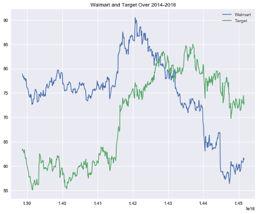
In the above plot, we can see a slight correlation at the beginning of 2014. But this doesn't really give us a clear idea of the relationship between Walmart and Target. To get a definitive idea of the relationship between the two stocks, we'll create a correlation heat-map.
To begin creating our correlation heatmap, we must first place Walmart and Target prices in the same dataframe. Let's create a new dataframe for our stocks.
#initializing newDF as a pandas dataframe
newDF=pd.DataFrame()
#adding WMT closing prices as a column to the newDF
newDF['WMT']=wmt['Close']
#adding TGT closing prices as a column to the newDF
newDF['TGT']=tgt['Close']
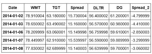
Now that we have created a new dataframe to hold our Walmart and Target stock prices, let's take a look at it.
newDF.head()
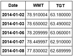
We can see that we have the prices of both our stocks in one place. We are now ready to create a correlation heatmap of our stocks. To this, we will use python's Seaborn library. Recall that we imported Seaborn earlier as sns.
#using seaborn as sns to create a correlation heatmap of WMT and TGT
sns.heatmap(newDF.corr())
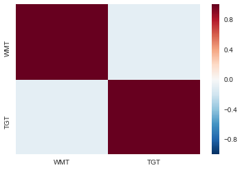
In the above plot, we called the corr() method on our newDF and passed it into Seaborn's heatmap object. From this visualization, we can see that our two stocks are not that correlated. Let's create a final visualization to asses this relationship. We'll use a scatter plot for this.
Earlier we used Matplotlibs scatter plot method. So now we'll introduce Seaborn's scatter plot method. Note that Seaborn is built on top of Matplotlib and thus matplotlibs functionality can be applied to Seaborn.
#Creating a scatter plot using Seaborn
plt.figure(figsize=(15,10))
sns.jointplot(newDF['WMT'],newDF['TGT'])
plt.legend(loc=0)
plt.show()
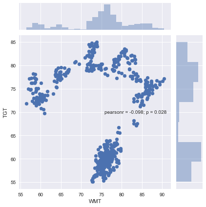
One feature that I like about using Seaborn's scatter plot is that it provides the Correlation Coefficient and P-Value. From looking at this pearsonr value, we can see that WMT and TGT were not positively correlated over the period. Now that we have a better understanding of our two stocks, let's check to see if a tradable relationship exists.
We'll use the Augmented Dickey Fuller Test to determine of our stocks can be traded within a Statistical Arbitrage Strategy.
Recall that we imported the adfuller test from the statsmodels.tsa.api package earlier.
To perform the ADF test, we must first create the spread of our stocks. We add this to our existing newDF dataframe.
#adding the spread column to the nemDF dataframe
newDF['Spread']=newDF['WMT']-newDF['TGT']
#instantiating the adfuller test
adf=adfuller(newDF['Spread'])
We have now performed the ADF test on our spread and need to determine whether or not our stocks are cointegrated. Let's write some logic to determine the results of our test.
#Logic that states if our test statistic is less than
#a specific critical value, then the pair is cointegrated at that
#level, else the pair is not cointegrated
if adf[0] < adf[4]['1%']:
print('Spread is Cointegrated at 1% Significance Level')
elif adf[0] < adf[4]['5%']:
print('Spread is Cointegrated at 5% Significance Level')
elif adf[0] < adf[4]['10%']:
print('Spread is Cointegrated at 10% Significance Level')
else:
print('Spread is not Cointegrated')
Spread is not Cointegrated
The results of the Augmented Dickey Fuller Test showed that Walmart and Target were not cointegrated. This is determined by a test statistic that is not less than one of the critical values. If you would like to view the actual print out of the ADF test you can do so by keying ADF. In the above example, we use indexing to decipher between the t-statistic and critical values. The statsmodels ADF Test provides you with other useful information such as the p-value. You can learn more about the ADF test here
#printing out the results of the adf test
adf
(-0.38706825965317432,
0.91223562790079438,
0,
503,
{'1%': -3.4434175660489905,
'10%': -2.5698395516760275,
'5%': -2.8673031724657454},
1190.4266834075452)
Okay, let's try one more. Maybe we'll have better luck identifying a tradable relationship in a brute force manner. How about Dollar Tree and Dollar General. They're both discount retailers and look they both even have a dollar in their names. Since we've gotten the hang of things, we jump right into the ADF test. Let's first import the data for DLTR and DG.
#importing dltr and dg
dltr=pdr.get_data_yahoo('DLTR',start, end)
dg=pdr.get_data_yahoo('DG',start, end)
Now that we've gotten our data, let's add these stocks to our newDF and create their spread.
#adding dltr and dg to our newDF dataframe
newDF['DLTR']=dltr['Close']
newDF['DG']=dg['Close']
#creating the dltr and dg spread as a column in our newDF dataframe
newDF['Spread_2']=newDF['DLTR']-newDF['DG']
We've now added the DLTR and DG stocks as well as their spread to our newDF dataframe. Let's take a quick look at our dataframe.
newDF.head()
Now that we have Spread_2 or the spread of DLTR and DG, we can create ADF2 or a second ADF test for these two stocks.
#Creating another adfuller instance
adf2=adfuller(newDF['Spread_2'])
We've just run the ADF test on our DLTR and DG spread. We can now repeat our earlier logic to determine if the spread yields a tradable relationship.
if adf2[0] < adf2[4]['1%']:
print('Spread is Cointegrated at 1% Significance Level')
elif adf2[0] < adf2[4]['5%']:
print('Spread is Cointegrated at 5% Significance Level')
elif adf2[0] < adf2[4]['10%']:
print('Spread is Cointegrated at 10% Significance Level')
else:
print('Spread is not Cointegrated')
Spread is not CointegratedTo view the complete print out of the ADF2 test, we can call adf2.
adf2
(-1.9620694402101162,
0.30344784824995258,
1,
502,
{'1%': -3.4434437319767452,
'10%': -2.5698456884811351,
'5%': -2.8673146875484368},
1305.4559226426163)
How about we take a breather here and review what we have learned so far. In this section, we began our journey toward understanding the efficacy of K-Means for pair selection and Statistical Arbitrage by attempting to develop a Statistical Arbitrage strategy in a world with no K-Means.
We learned that in a Statistical Arbitrage trading world without K-Means, we are left to our own devices for solving the historic problem of pair selection. We've learned that despite two stocks being related on a fundamental level, this doesn't necessarily insinuate that they will provide a tradable relationship.
In the next section, we will get a better understanding of K-Means and then prepare to apply it to our own Statistical Arbitrage strategy.
Understanding K-Means
Before we start implementing the K-means clustering algorithm for statistical arbitrage, let's take a look at how K-Means works.
We will begin by importing our usual data analysis and manipulation libraries. Sci-kit learn offers built-in datasets that you can play with to get familiar with various algorithms. You can take a look at some of the datasets provided by sklearn here.
To gain an understanding of how K-Means works, we're going to create our own toy data and visualize the clusters. Then we will use sklearn's K-Means algorithm to assess its ability to identify the clusters that we created. Let’s get started!
#importing necessary libraries
#data analysis and manipulation libraries
import numpy as np
import pandas as pd
#visualization libraries
import matplotlib.pyplot as plt
import seaborn as sns
#machine learning libraries
#the below line is far making fake data far illustration purposes
from sklearn.datasets import make_blobs
Now that we have imported our data analysis, visualization and the make_blobs method from sklearn, we're ready to create our toy data to begin our analysis.
#creating fake data
data=make_blobs(n_samples=500, n_features=8,centers=5, cluster_std=1.5, random_state=201)
In the above line of code, we have created a variable named data and have initialized it using our make_blobs object imported from sklearn. The make blobs object allows us to create and specify the parameters associated with the data we're going to create. We're able to assign the number of samples, or the number of observations equally divided between clusters, the number of features, clusters, cluster standard deviation, and a random state. Using the centres variable, we can determine the number of clusters that we want to create from our toy data.
Now that we have initialized our method, let's take a look at our data.
#Let's take a look at our fake data
data[0] #produces an array of our samples
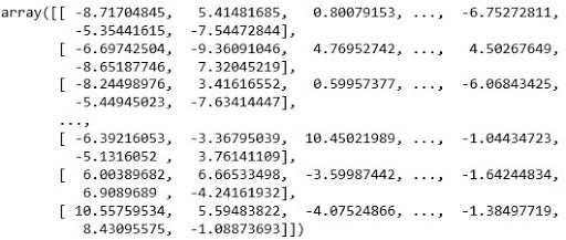
Printing data[0] returns an array of our samples. These are the toy data points we created when initializing the n_samples parameter in our make_blobs object. We can also view the cluster assignments we created.
#viewing the clusters of our data
data[1]
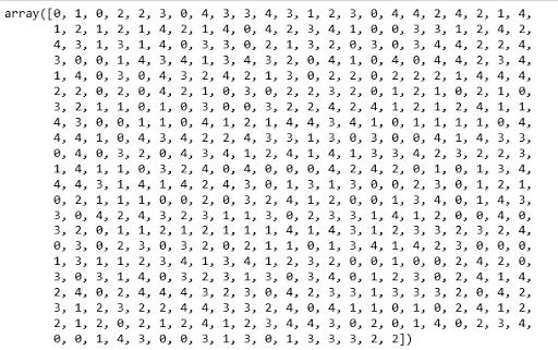
Printing data[1] allows us to view the clusters created.
Note that though we specified five clusters in our initialization, our cluster assignments range from 0 to 4. This is because python indexing begins at 0 and not 1. So cluster counting, so to speak, begins at 0 and continues for five steps.
We've taken a look at our data and viewed our clusters, but looking at arrays doesn't give us a lot of information. This is where our visualization libraries come in. Python's matplotlib is a great library for visualizing data so that we can make inferences about it. Let's create a scatter plot, or a visual to identify the relationships inherent in our data.
#creating a scatter plot of our data in features 1 and 2
plt.scatter(data[0][:,0],data[0][:,1])
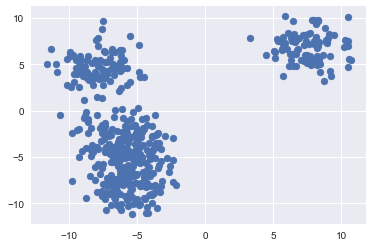
The above plot gives us a little more information. Not to mention its easier to read. We have created a scatter plot of our sample data using the first two features we created. We can somewhat see that there are some distinct clusters. The group to the upper right of the chart is the most distinct. There is also a degree of separation in the data to the left of the chart. But, didn't we assign five clusters to our data? We can't visually see the five clusters yet, but we know that they're there.
One way that we can improve our visualization is to colour it by the clusters we created.
#the above plot doesn't give us much information
#Let's recreate it using our clusters
plt.scatter(data[0][:,0],data[0][:,1],c=data[1])
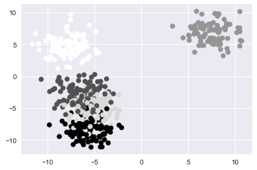
The above plot is an improvement. We can now see that the grouping to the lower left of our original plot was actually multiple overlapping clusters. What would make this visualization even better is if we added more distinct colours that would allow us to identify the specific points in each cluster. We can do this by adding another parameter to our scatter plot called cmap. The cmap parameter will allow us to set a colour mapping built into matplotlib to recolour our data based on our clusters. Learn more about matplotlib's colour mapping.
#we can improve the above visualization by adding a color map to our plot
plt.scatter(data[0][:,0],data[0][:,1],c=data[1],cmap=‘gist_rainbow')
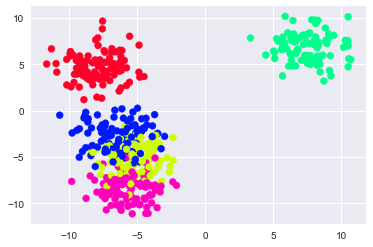
To review, at this point, we have created some toy data using sklearn's built-in make_blobs method. We then viewed the rows of the first two features, followed by the actual clusters of our toy data. Next, we plotted our data both with and without colouring based on the clusters.
To display how K-Means is implemented, we can now create the K-Means object and fit it to our toy data and compare the results.
#importing K-Means
from sklearn.cluster import KMeans
Each time that we import a model in sklearn, to use it, must create an instance of it. The models are objects and thus we create an instance of the object and specify the parameters for our specific object.
Naturally, this allows us to create a variety of different models, each with different specifications for our analysis. In this example, we'll create a single instance of the K-Means object and specify the number of clusters.
#instantiating K-means
model=KMeans(n_clusters=5) #n_clusters represents # of clusters; we know this because we created this dataset
KMeans(algorithm='auto', copy_x=True, init='k-means++', max_iter=300,
n_clusters=5, n_init=10, n_jobs=1, precompute_distances='auto',
random_state=None, tol=0.0001, verbose=0)
In the above line of code, we have now fitted our model to our data. We can see that it confirms the parameters our model applied to our data.
Next, now that we have both our toy data and have visualized the clusters we created, we can compare the clusters we created from our toy data to the ones that our K-Means algorithm created based on viewing our data.
We'll code a visualization similar to the one we created earlier, however, instead of a single plot, we will use matplotlibs subplot method to create two plots, our clusters and K-Means clusters, that can be viewed side by side for analysis. If you would like to learn more about matplotlibs subplot functionality, you can visit here.
#now we can compare our clustered data to that of K-means
#creating subplots
plt.figure(figsize=(10,8))
plt.subplot(121)
plt.scatter(data[0][:,0],data[0][:,1],c=data[1],cmap='gist_rainbow')
#in the above line of code, we are simply replotting our clustered data
#based on already knowing the labels(i.e. c=data[1])
plt.title('Our Clustering')
plt.tight_layout()
plt.subplot(122)
plt.scatter(data[0][:,0],data[0][:,1],c=model.labels_,cmap='gist_rainbow')
#notice that the above line of code differs from the first in that
#c=model.labels_ instead of data[1]...this means that we will be plotting
#this second plot based on the clusters that our model predicted
plt.title('K-Means Clustering')
plt.tight_layout()
plt.show()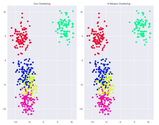
The above plots show that the K-Means algorithm was able to identify the clusters within our data. The colouring has no bearing on the clusters and is merely a way to distinguish clusters.
In practice, we won't have the actual clusters that our data belongs to and thus we wouldn't be able to compare the clusters of K-Means to prior clusters; But what this walkthrough shows is the ability of K-Means to identify the presence of subgroups within data.
At this point in our journey toward better understanding the application and usefulness of K-Means, we’ve created our own clusters from data we created, used the K-Means algorithms to identify the clusters within our toy data and travelled back in time to a Statistical Arbitrage and mean reversion trading world with no K-Means
Let’s pause for a moment and understand what we have learnt so far. We know that K-Means assigns data points to clusters randomly initially and then calculates centroids or mean values. Further, it calculates the distances within each cluster, squares these, and sums them, to get the sum of squared error.
The goal is to reduce this error or distance. The algorithm repeats this process until there is no more in-cluster variation, or put another way, the cluster compositions stop changing.
Great! Now, where do we go from here? Well, in the next section, we will enter a Statistical Arbitrage trading world where K-Means is a viable option for solving the problem of pair selection and use the same to implement a Statistical Arbitrage trading strategy.
To Begin, we need to gather data for a group of stocks. We'll continue using the S&P 500. There are 505 stocks in the S&P 500. We will collect some data for each of these stocks and use this data as features for K-Means. We will then identify a pair within one of the clusters, test it for cointegration using the ADF test, and then build a Statistical Arbitrage trading strategy using the pair.
Let’s dive right in!
Building A StatArb Strategy Using K-Means
We'll begin by reading in some data from an Excel File containing the stocks and features will use.
#Importing Our Stock Data From Excel
file=pd.ExcelFile('KMeansStocks.xlsx')
#Parsing the Sheet from Our Excel file
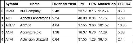
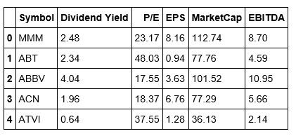
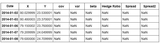
stockData=file.parse('Example')Now that we have imported our Stock Data from Excel, let's take a look at it and see what features we will be using to build our K-Means based Statistical Arbitrage Strategy.
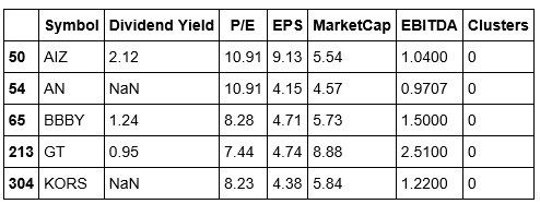
#Looking at the head of our Stock Data
stockData.head()
#Looking at the tail of our Stock Data
stockData.tail()
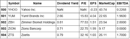
We're going to use the Dividend Yield, P/E, EPS, Market Cap, and EBITDA as the features for creating clusters across the S&P 500. From looking at the tail of our data, we can see that Yahoo doesn't have a Dividend Yield, and is missing the P/E ratio. This brings up a good teaching moment. In the real world, data is not always clean and thus will require that you clean and prepare it so that it's fit to analyze and eventually use to build a strategy.
In actuality, the data imported has been preprocessed a bit as I've already dropped some unnecessary columns from it.
Process Of Implementing A Machine Learning Algorithm
Let's take a moment and think about the process of implementing a machine learning algorithm.
- We begin by collecting our data
- Next, we want to make sure our data is clean and ready to be utilized
- In some cases, dependent upon what algorithm we're implementing, we conduct a train-test split( for K-Means this isn't necessary)
- After conducting the train-test split, we then train our algorithm on our training data and then test it on our testing data
- We then survey our model's precision
Implementation
Let's begin by cleaning up our data a little more. Let's change the index to the Symbols column so that we can associate the clusters with the respective symbols. Also, let's drop the Name column as it serves no purpose.
Before making additional changes to our data, let's make a copy of our original. This is a good practice as we could incur an error later and will be able to reset our implementation if we are working with a copy of the original instead of the original.
#Making a copy of our stockdata
stockDataCopy=stockData.copy()
#Dropping the Name column from our stockData
stockDataCopy.drop('Name', inplace=True,axis=1)
It's a good practice to go back and check your data after making changes. Let's take a look at our stockData to confirm that we properly removed the Name column. Also, in the above line of code, we want to be sure that we include inplace=True. This states that the changes will persist in our data.
#Checking the head of our stockData
stockDataCopy.head()

Okay, now that we have properly dropped the Name column, we can change the index of our data to that of the Symbol column.
stockDataCopy.reindex(index=stockDataCopy['Symbol'],columns=stockDataCopy.columns)
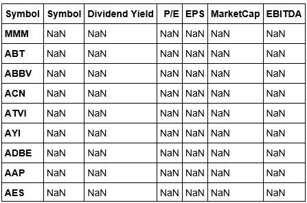
We've reindexed our stockData, but this view isn't exactly what we were expecting. Let's fix this by adding the values back to our columns. We are able to do this because we are working using a copy of our original.
#Adding back the values to our Columns
stockDataCopy['Symbol']=stockData['Symbol'].values
stockDataCopy['Dividend Yield']=stockData['Dividend Yield'].values
stockDataCopy['P/E']=stockData['P/E'].values
stockDataCopy['EPS']=stockData['EPS'].values
stockDataCopy['MarketCap']=stockData['MarketCap'].values
stockDataCopy['EBITDA']=stockData['EBITDA'].values
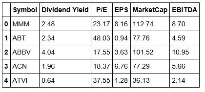
We've added the data back to our stockDataCopy dataframe. Note in the code above, we were able to this because we could simply port over the values from our original dataframe. Let's take another look at our stock data.
#Viewing the head of our stockDataCopy dataframe
stockDataCopy.head()
It appears that Jupyter Notebook responds differently to reindexing and reassigning values to our dataframe that of the Spyder IDE. We won't worry about this for now but may need to create a workaround in the future. Now we will focus on clustering our data. We begin by instantiating another K-Means object.
stock_kmeans=KMeans()
Wait, How Do We Find K???
This brings us to another critical component of our strategy development. Recall, in our example of K-Means clustering, we created our own toy data and thus were able to determine how many clusters we would like. When testing the K-Means algorithm, we were able to specify K as 5 because we knew how many clusters it should attempt to create.
However, working with actual data, we are not aware of how many subgroups are actually present in our stock data. This means that we must identify a means of determining the appropriate amount of clusters, or value for K, to use.
One such technique is to use termed the 'elbow' technique. We've mentioned this earlier, but I'll briefly recap. We plot the number of clusters versus the sum of squared errors, or SSE. Where the plot tends to bend, forming an elbow like shape, is the value of the clusters that we should select.
So, what we are tasked with doing, is to create a range of values for K, iterate over that range, and at each iteration fit our stock_kmeans model to our data. We will also need to store our K values and have a way to calculate the distances from the centroids of each iteration so that we can compute our SSE or sum of squared errors.
To find our distances, we'll use scipy. Let's import it now.
from scipy.spatial.distance import cdist
If you would like to learn more about the cdist object you can visit this link.
The distance used in K-Means is the Euclidean distance and this is the one we will use with this method.
Let's create our elbow chart to determine the value of K.
#creating an object to determine the value for K
class Get_K(object):
def __init__(self,start,stop,X):
self.start=start
self.stop=stop
self.X=X
#in our example, we found out that there were some NaN
#values in our data, thus we must fill those with 0
#before passing our features into our model
self.X=self.x.fillna(e)
def get_k(self):
#this method will iterate through different
#values of K and create the SSE
#initializing a list to hold our error terms
self.errors=[ ]
#intializing a range of values for K
Range=range(self.start,self.stop)
#iterating over range of values far K
#and calculating our errors
for i in Range:
self.k_means=KMeans(n_clusters=i)
self.k_means.fit(self.X)
self.errors.append(sum(np.min(cdist(self.X[0:200],self.k_means.cluster_centers_,'euclidean'),axis=1))/200)
return
 def plot_elbow(self):
with plt.style.context(['seaborn-notebook','ggplot‘]):
plt.figure(figsize=(10,8))
#we have multiple features, thus we will use the
#P/E to create our elbow
plt.plot(self.X['P/E'][0:200],self.errors[0:200])
plt.xlabel('Clusters')
plt.ylabel('Errors')
plt.title('K-Means Elbow Plot')
plt.tight_layout()
plt.show()
Return
We now have an object to determine the value we should use for K. We will create an instance of this object and pass in our stockData and determine the value we should use for K.
Let's first create a list of our features.
features=stockDataCopy[[‘Dividend Yield','P/E','EPS','MarketCap','EBITDA']]
Now that we have set our features, we can pass them into our K-Means algorithm.
#Creating an instance of our Get_K object
#we are setting our range of K from 1 to 266
#note we pass in the first 200 features values in this example
#this was done because otherwise, to plot our elbow, we would
#have to set our range max at 500. To avoid the computational
#time associated with the for loop inside our method
#we pass in a slice of the first 200 features
#this is also the reason we divide by 200 in our class
Find_K=Get_K(1, 200,features [1:200]
At this point, we have created our list of features, and have created an instance of our Get_K class with a possible range of K from 1 to 200.
Now we can call our get_k method to find our errors.
#Calling get_k method on our Find_K object
Find_K.get_k()
Visualizing K-Means Elbow Plot
Now that we have used our get_k method to calculate our errors and range of K, we can call our plot_elbow method to visualize this relationship and then select the appropriate value for K.
#Visualizing our K-Means Elbow Plot
Find_K.plot_elbow()
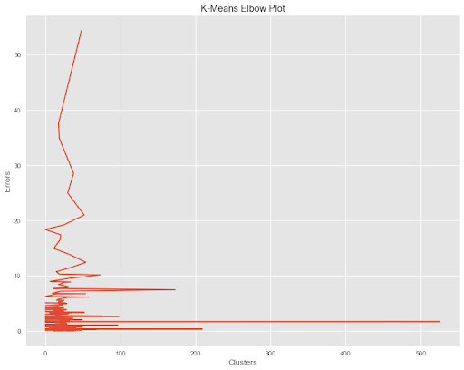
We can now use the above plot to set our value for K. Once we have set K, we can apply our model to our stock data and then parse out our clusters and add them back to our stockData dataframe. From here we are then able to manipulate our dataframe so that we can identify which stocks are in which cluster. Afterwards, we can select pairs of stocks and complete our analysis by checking to see if they are cointegrated and if so build out a Statistical Arbitrage strategy.
Let’s take a break here and look back at the knowledge we have gained so far. We have continued to build on our understanding of how K-Means can improve our Statistical Arbitrage strategies. We learned that an important problem to solve with implementing K-Means is determining what value we should use for K.
We've covered a lot and now we're almost to the point we've been waiting for, coding our strategy. Let’s start right away!
K-Means StatArb Implementation
We're going to create a class that will allow us to clean our data, test for cointegration, and run our strategy simply by calling methods off of our Statistical Arbitrage object.
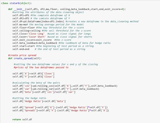
Let's briefly walk through what the above code does.
We begin by creating an instance of our statarb class. We pass in the two dataframes of the two stocks that we want to trade along with parameters for the moving average, the floor or buy level for z-score, the ceiling, or sell level for z-score, the beta lookback period for our hedge ratio, and our exit level for our z-score. By default, this level is set to 0.
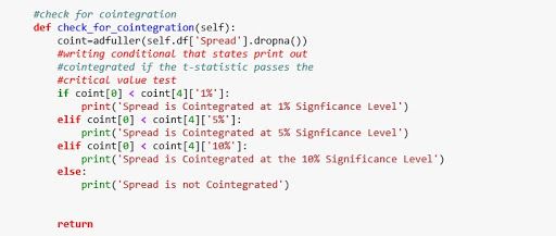
Once we've created our stat arb object, we can then access its methods. We begin by cleaning our data within our create spread method as we did earlier. Once our data has been clean, we can then call our check for cointegration method. This method will take the spread created in our create spread method and then pass it into the ADF test and return whether or not the two stocks are cointegrated.
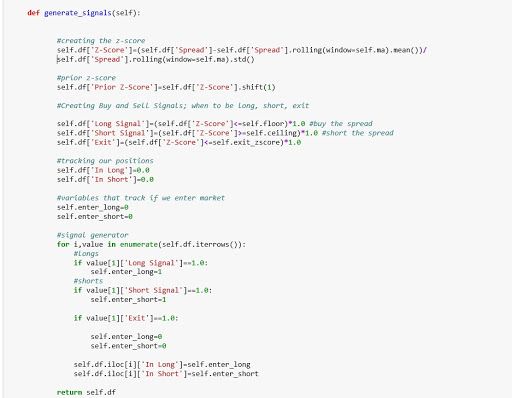
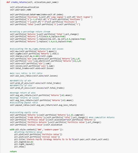
If our stocks are cointegrated, we can then call our generate signals method which will implement the Statistical Arbitrage strategy. From here we can call our create returns method. This method will require that we pass in an allocation amount. This is the amount of our hypothetical portfolio and will be used to create our equity curve. After our equity curve is created, we will then have access to other data such as our hit ratio, wins and losses, and our Sharpe ratio.
To implement the strategy, we must keep track of our current position while iterating over the dataframe to check for signals. For a good walkthrough of how to implement the Statistical Arbitrage strategy, visit Quantstart.com. Here's the link to the article. Michael does a great job providing insight into each step of the implementation.
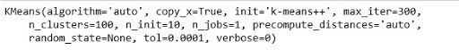
We'll set K equal to 100. Let's begin by instantiating our K-Means object.
![]()
Now let's fit our model on the features of our data.
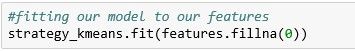
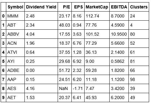
Now that we have fitted our model to our features, we can get our clusters and add them to our stockDataCopy dataframe. Also, note that we called the fillna() method on our features. This was done because we noticed that some of our features had NaN values and this can't be passed into our model. We didn't call dropna() to drop these values as this would have changed the length of our features and would present issues when adding the clusters back to our dataframe.
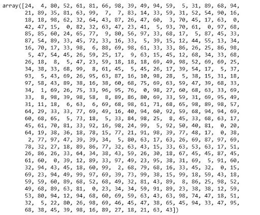
Let's take a look at our clusters.
![]()
Okay now that we have our clusters, we can add them back to our data. Let's first take another look at our dataframe.
Let's add a column for our clusters to our dataframe.
![]()
Let's review our dataframe once more.
![]()
Now that we have our clusters in our dataframe, our next task is to identify tradable pairs within our clusters.
Let's take a look at how many stocks were placed in each cluster. To do this we will import the Counter method from the collections library.
![]()
![]()
Now that we have created a variable to count the number of symbols in each cluster, we can print it.
![]()
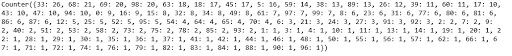
Now we are ready to add our clusters to our dataframe. But, notice above, when looking at how many values are in each of our clusters, we can see that some clusters only have 1 symbol. We would like to eliminate these and only view clusters that have 2 or more symbols within them. We would also like to order our data by cluster so that we can view every symbol within a respective cluster.
To achieve this we will create a new dataframe and use pandas concat method to concatenate it with our stockDataCopy dataframe grouped according to the Clusters column but filter out those clusters contain less than 2 symbols.
![]()
We can save our concatenation into a variable that will allow us to perform the operation on it.
![]()
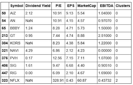
![]()
The above dataframe shows us five symbols in Cluster 0. We can see that the index represents their original position in our stock dataframe. We’re also able to make a brief comparison of their features.
We can now see scroll or iterate through our dataframe and see which symbols are in each cluster with the minimum being at least two symbols. Let's use our statarb method to test a pair of symbols for cointegration and develop a Statistical Arbitrage strategy.
We will begin by creating an instance of our statarb object. We will randomly select two stocks from cluster 0 for this analysis. We must first import the data for each symbol over our testing period.
Now that we have imported our data, let's take a quick look at it.
Okay now, let's test our statarb class to test the symbols for cointegration and build a strategy.
![]()
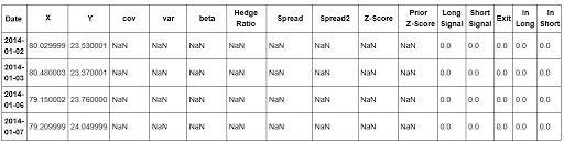
Okay in the above line of code, we have just created an instance of our statarb strategy class. We can now call our create_spread method to create the spread of our data. We passed in the entire dataframes of bbby and gt because this method will parse the closing prices and created the spread for us. Afterwards, we can call the remaining methods to complete our Statistical Arbitrage analysis.
![]()
In the above dataframe, we can see that we’ve added our spread. The values at the head are NaN which is reflective of the lookback that we are using. We can scroll down to see that values have been populated for each column.
Now that we have created the spread of our pair, let's check to see if they are cointegrated.
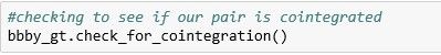
![]()
Our pair is highly cointegrated. Now that we have confirmed this, we can call our generate signals and create returns to see how our strategy would have performed over our testing period.
![]()
We can see that we have added our signals to our dataframe.
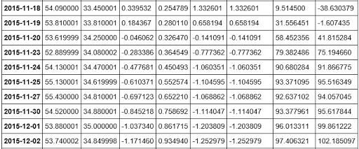
Now that we have generated signals for our pair, let's use our create returns method to calculate our returns and print our equity curve. Recall that this method takes in an allocation amount. This is the starting value of our portfolio. This method also requires that we pass in a name for our pair as a string to be included in our plot.
![]()
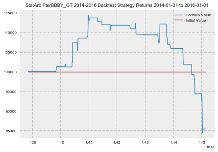
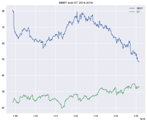
We can see that our strategy did well for a while before appearing to no longer be cointegrated. Let's take a look at our Sharpe Ratio.
![]()
Challenge: See If You Can Improve This Strategy
Try your hand at improving this strategy. Our analysis showed that these two stocks were highly cointegrated. However, after performing well for the majority of our testing period, the strategy appears to have loss cointegration.
This shows a couple of things.
- It shows that Statistical Arbitrage is not a riskless trading strategy.
- It underscores the importance of the parameters used when trading. These are what are truly proprietary.
Conclusion
Wow! We have covered an immense amount of information in a short time. To recap, we began by gaining an understanding of K-Means. We also took a walk through a Statistical Arbitrage world without K-Means. We brute-forced the creation of a couple of pairs and learned that identifying tradeable relationships involved a little more than finding pairs in the same sector. We then used real stock data from the S&P 500, namely Dividend Yields, P/E, MarketCap, EPS and EBITDA, as features to begin creating a real-world K-Means analysis for trading Statistical Arbitrage.
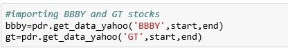
We then added our clusters to our dataframe and manipulated it so that we could test the pairs in each cluster for cointegration via the ADF test. We randomly selected BBBY and GT from cluster 0 of our analysis and found that they were cointegrated at the 99% significance level. Afterwards, we used the statarb class we created to backtest our new found pair. Whew!
This analysis also showed the strength of K-Means for finding non-traditional pairs for trading Statistical Arbitrage. BBBY is the ticker symbol of Bed Bath and Beyond and GT is the ticker symbol for Goodyear Tire & Rubber Co. These two stocks appear to have nothing in common on the surface but have been cointegrated at the 1% critical value in the past.
Next Step
If you want to learn various aspects of Algorithmic trading then check out the Executive Programme in Algorithmic Trading (EPAT™). The course covers training modules like Statistics & Econometrics, Financial Computing & Technology, and Algorithmic & Quantitative Trading. EPAT™ equips you with the required skill sets to be a successful trader. Enroll now!
Disclaimer: All investments and trading in the stock market involve risk. Any decisions to place trades in the financial markets, including trading in stock or options or other financial instruments is a personal decision that should only be made after thorough research, including a personal risk and financial assessment and the engagement of professional assistance to the extent you believe necessary. The trading strategies or related information mentioned in this article is for informational purposes only.
Download Python Code
- Python Code for Building a StatArb Strategy Using K-Means
