This article is the final project submitted by the author as a part of his coursework in Executive Programme in Algorithmic Trading (EPAT®) at QuantInsti®. Do check our Projects page and have a look at what our students are building.
About the Author

Javier Cervantes, CFA
Javier Cervantes is currently a corporate bond trader at BCP Securities, specializing in MXN-denominated debt. He is also a CFA charterholder, having obtained his charter in August, 2017. Javier holds a BS in Economics from Instituto Tecnológico Autónomo de México (ITAM).
Project
There are very few algo trading firms/strategies that are operating in the Mexican stock exchange. I believe this should provide great opportunities as there is little competition. Contrary to a more developed market, arbitrage opportunities aren’t readily realized which suggests there might be opportunities for those looking and able to take advantage of them.
This is the main motivation for this strategy and the main reason I reached out to Quantinsti. As there are few players involved, learning about algo trading can potentially set me up for great opportunities in the future.
The fact that the Mexican market is not as developed will also create certain complications. There are around 200 listed companies on the Mexican stock exchange. Of that, I’ve filtered those with incomplete information (using Google Finance) to arrive at a universe of 117 stocks (see attached Excel “Emisoras BMV.xlsx”) which will be further filtered and cleaned to meet certain conditions.
The trading strategy implemented in this project is called “Statistical Arbitrage Trading”, also known as “Pairs Trading” which is a contrarian strategy designed to profit from the mean-reverting behavior of a certain pair ratio. The assumption behind this strategy is that the spread from pairs that show properties of cointegration is mean-reverting in nature and therefore will provide arbitrage opportunities if the spread deviates significantly from the mean.
The trading strategy will be back-tested for the period between 01/01/2012 and 30/06/2017. This period will be divided into an in-sample back-test which will run between 01/01/2012 and 31/12/2015 and the remainder which will be used for the out-of-sample backtest.
Before defining the strategy, I have to determine which stocks will be eligible for trading. For this, I shall establish daily trading volume, cointegration, and correlation limits. Once the stock universe has been cleaned, the back-testing can begin.
Given the chosen universe of stocks, I shall first apply a filter for those that don’t have complete daily prices for the given time horizon. Once those stocks are eliminated, I’ve set a minimum average daily trading volume of 15 million pesos (MXN) to be eligible for trading.
Now that stocks have been filtered for their data and daily liquidity, every possible stock pair for each industry will be tested for cointegration. An ADF test will be performed such that, the alternative hypothesis is that the pair to be tested is stationary. The null hypothesis will be rejected for p-values <0.025.
The final filter to be used is the correlation. Those pairs with a correlation coefficient lower than 0.60 will be eliminated. The following pairs are the ones that made the cut:

The following is a scatter-plot from the prices of each one of the remaining pairs that will be used in the trading strategy:

Now, zscores will be created for every price ratio that remains. The time horizon used in the moving average and standard deviation calculations to build the zscores is 60 days. This is how the zscore graphs with +2/-2 standard deviation lines look:
 The trading strategy will consist of creating a primary sell signal for the pair ratio (short the relatively expensive stock and simultaneously buy the relatively cheap stock) if the pair is trading between 2 and 2.25 standard deviations above the mean, at which point, 75% of the available risk capital for that ratio will be sold. A secondary sell signal for the pair ratio appears for the remaining 25% of risk capital if the pair’s zscore crosses 2.25 standard deviations. An analogous primary buy and secondary buy signals are created when the pair is trading below 2 and 2.25 standard deviations respectively below the mean. The usefulness of the two-step entry signals will be evaluated using the Sharpe ratio of the aggregate results once the backtesting is complete. Each trade’s exit signal will be triggered once the pair’s zscore crosses 0.
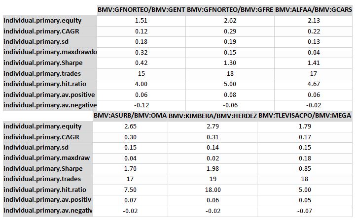
If one were to treat each pair as an individual trade, here are the results that would’ve been obtained:

As one can see, results vary considerably between pairs. Maximum drawdown ranges from a low of 2% to a high of 32%. CAGR ranges from 12% to 31%. If the returns correlation of each pair is low, the strategy could benefit from diversification. Let’s take a look at the correlation matrix:

This is the equity curve that was generated for each one of the pairs analyzed previously:

Allocating one’s entire risk capital to a single pair might be too risky. Given that the observed correlations between pairs are relatively low, let’s analyze the following strategy: we’ll now assume that every remaining pair receives the same initial risk capital allocation.
First, we analyze primary and secondary trades separately and test to see if we gain from implementing the separate (primary & secondary) entry signals. A portfolio’s Sharpe ratio will improve from adding a new instrument if the following condition is met:

Evaluating the previous expression results in 2.41>2.12; since this condition is true, running the strategy using both entry signals will result in a higher Sharpe ratio for this trading strategy.
These are the final results from the complete trading strategy:

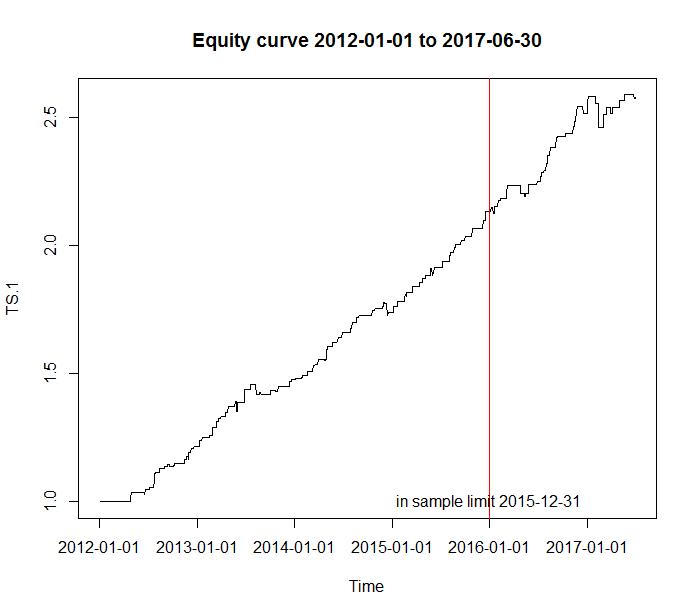
First to be noted is that the in-sample Sharpe ratio (2.79) is higher than that which was calculated earlier using only primary signal trades (2.41). Second, the max drawdown on this strategy is considerably low which allows for significant flexibility in the use of leverage. Third, we can observe that the out-of-sample results are lower but still offer exceptional risk-adjusted returns.
Here is the equity curve generated from this strategy:

There is no direct comparison to use for the results presented above but we can estimate the correlation of this strategy with Mexico’s stock market index, the IPC (google ticker “INDEXBMV:ME”). Over the in-sample data, the correlation coefficient is 0.62 which could provide diversification benefits to a “market portfolio”. Another strategy that can implement this model is “equitizing a market-neutral long-short portfolio”. This strategy consists in following a passive investment strategy using futures of the market index (with a notional equivalent to the reserve cash position needed to short stock) and looks to generate some alpha with our statistical arbitrage strategy.
Conclusions:
There are significant opportunities to be seized in the Mexican stock market with strategies suited for many types of investors.
One must also realize there are yet a few things to be considered before implementing this trading strategy; many will depend on the investor type:
- Given the low maximum drawdown observed in this strategy, the prudent use of leverage can further enhance the previous results
- The previous results don’t account for implicit and explicit trading costs
- Further back-testing, particularly in different time periods is recommended to get a better handle on the performance of this trading strategy in different market conditions. One can also test the strategy using different values for variables like entry levels, risk capital allocation, time horizon, correlation and confidence level on the ADF test
- As with the two-step entry signals, one can test the results using multi-step exit strategies. Of particular importance will be the implementation of stop losses that can be based on different levels of zscore, correlation, volatility, etc
- The assumption is that all of the stocks used in the strategy can be shorted. Complications might arise in the actual implementation of the strategy.
Bibliography:
CHAN, Ernest. Algorithmic Trading, Winning Strategies, and their Rationale.
TSAY, Ruey. Analysis of Financial Time Series
QUANTINSTI. Statistical Arbitrage (Pair Trading & Index Arbitrage) lecture
Next Step
If you want to learn various aspects of Algorithmic trading then check out the Executive Programme in Algorithmic Trading (EPAT™). The course covers training modules like Statistics & Econometrics, Financial Computing & Technology, and Algorithmic & Quantitative Trading. EPAT™ equips you with the required skill sets to build a promising career in algorithmic trading. Enroll now!
Update
We have noticed that some users are facing challenges while downloading the market data from Yahoo and Google Finance platforms. In case you are looking for an alternative source for market data, you can use Quandl for the same.
Disclaimer: The information in this project is true and complete to the best of our Student’s knowledge. All recommendations are made without guarantee on the part of the student or QuantInsti®. The student and QuantInsti® disclaim any liability in connection with the use of this information. All content provided in this project is for informational purposes only and we do not guarantee that by using the guidance you will derive a certain profit.
Files in the download:
- Emisoras BMV.csv
- Pairs trading BMV Mex .R


