In the previous blogs, we examined supervised learning algorithms like linear regression in detail. In this blog, we look at what unsupervised learning is and how it differs from supervised learning.
Then, we move on to discuss some use cases of unsupervised learning in investment and trading. We explore two unsupervised techniques in particular- k-means clustering and PCA with examples in Python.
Contents
- What is unsupervised learning?
- Supervised vs unsupervised learning
- When do we use unsupervised algorithms?
- Clustering algorithms
- Concept of clustering
- K-means clustering algorithm
- Dimensionality Reduction
- Concept of dimensionality reduction
- Principal Component Analysis
- Other types of unsupervised algorithms
- Challenges in unsupervised learning
What is unsupervised learning?

As the name suggests, 'unsupervised' learning takes place when there is no supervisor or teacher and the learner learns on her own.
For instance, consider a child who sees and tastes an apple for the very first time. She registers the colour, the texture, the taste and the smell of the fruit. The next time she sees an apple, she knows that both this and the previous apple are similar objects as they have very similar characteristics.
She knows that this is very different from an orange. But still, she does not know what it is called in human-speak, i.e. an 'apple' as there is no knowledge of the label.
Such learning where the labels do not exist (in the absence of a teacher) but the learner can still learn about patterns on her own is referred to as unsupervised learning.
In the context of machine learning algorithms, unsupervised learning occurs when an algorithm learns from plain examples without any associated response and determines the data patterns on its own.
In the next section, we will discuss how this type of learning differs from the other type of popular learning algorithms in machine learning, i.e. supervised learning algorithms.
Artificial intelligence in trading leverages unsupervised learning to identify hidden patterns and trends within market data, enabling traders to uncover insights that may not be apparent through traditional analysis. This approach enhances the ability to develop adaptive trading strategies based on real-time market behavior.
Supervised vs unsupervised learning
Learning in supervised learning, as the name suggests, occurs under supervision, i.e., when the algorithm predicts a value for a sample from the training data, it is told whether the prediction was correct or not.
This is possible as we have the correct values stored as 'labels'/'target variable', which are passed to the algorithm along with the input data. Common supervised learning tasks are those of classification and regression.
In classification tasks, the labels are the correct class to which the sample belongs, whereas, in regression, the actual value of the dependent variable(Y) serves as a benchmark for comparing the prediction. The algorithm can then tweak its parameters to achieve higher accuracy in prediction.
Thus, the main goal of supervised learning is to build a robust predictive model.
On the other hand, in unsupervised learning, we only pass the input data, and there are no labels. Unsupervised models seek to find the underlying or hidden structure or distribution in the data in order to learn more about the data.
In other words, unsupervised learning is where we only have input data and no corresponding output variables, and the main goal is to learn more or discover new insights from the input data itself.
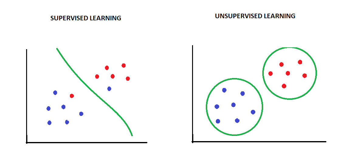
A common example of unsupervised algorithms are the clustering algorithms, that group the data based on the patterns that the machine detects.
For example, let us consider a situation in which we have a few data points based on two input features X1 and X2.
- If we want our algorithm to classify/categorize the data into two known classes, we will use a supervised classification algorithm.
- On the other hand, if we want the algorithm to tell us how the data is structured, we would use an unsupervised clustering algorithm.
When do we use unsupervised algorithms?
Unsupervised learning is utilized under the following conditions:
- We do not have the output/target data.
- We don’t exactly know what we are looking for and want the machine to discover patterns/insights in the data. The insights discovered by the machine can then be used to solve various challenges.
- We want to filter out only essential information(which has a lower dimension compared to original data) from the data and just use it to train a supervised learning model.
In the next two sections, we will look at two popular unsupervised algorithms, namely clustering and dimensionality reduction, which help us in these situations.
Clustering Algorithms
Concept of Clustering
Clustering is one of the most popular tasks in the domain of unsupervised learning. Here, the fundamental assumption is that the data points that are similar tend to belong to similar groups (called clusters), as determined by their distance from local centroids.
So rather than defining groups before looking at the data, clustering allows us to find and analyze the groups that have formed organically, i.e., based on the data itself.
There are different clustering algorithms such as K-means clustering, Hierarchical clustering, DBSCAN, OPTICS etc., which group the data according to their own definitions of similarity between the data points.
In the next subsection, we will look at an example of K-means clustering which is a widely used clustering algorithm. It creates 'K' similar clusters of data points.
K-means Clustering algorithm
K-means clustering is used when we have unlabeled data, i.e., data without defined categories or groups). This algorithm finds groups/clusters in the data, with the number of groups represented by the variable 'k'(hence the name).
The algorithm works iteratively to assign each observation to one of the k groups based on the similarity in provided features.
The inputs to the K-means algorithm are the data/features(Xis) and the value of 'K'(number of clusters to be formed).
The steps can be summarized as:
- The algorithm starts with randomly choosing 'K' data points as 'centroids', where each centroid defines a cluster.
- In this step, each data point is assigned to a cluster defined by a centroid such that the distance between that data point and the cluster's centroid is minimum.
- In this step, the centroids are recalculated by taking the mean of all data points that were assigned to that cluster in the previous step.
The algorithm iterates between steps (ii) and (iii) until a stopping criterion is met, such as a pre-defined maximum number of iterations are reached or datapoints stop changing clusters.
Example of K-means clustering for trading or investing with code in Python
Often, traders and investors want to group stocks based on similarities in certain features.
For example, a trader who wishes to trade a pair-trading strategy where she simultaneously takes a long and shorts position in two similar stocks would ideally want to scan through all the stocks and find those which are similar to each other in terms of industry, sector, market- capitalization, volatility or any other features.
Now consider a scenario where a trader whats to group/cluster stocks of 12 American companies based on two features:
- Return on equity (ROE) = Net Income/Total shareholder's equity, and
- The beta of the stock
Investors and traders use ROE to measure the profitability of a company in relation to the stockholders' equity. A high ROE is, of course, preferred to invest in a company. Beta, on the other hand, represents stock's volatility in relation to the overall market(represented by the index such as S&P 500 or DJIA).
Going through each and every stock manually and then forming groups is a tedious and time-consuming process. Instead, one could use a clustering algorithm such as the k-means clustering algorithm to group/cluster stocks based on a given set of features.
Below, we implement a K-means algorithm for clustering these stocks in Python. We start with importing the necessary libraries and fetching the required data using the following commands:
Downloaded: ADBE
Downloaded: AEP
Downloaded: CSCO
Downloaded: EXC
Downloaded: FB
Downloaded: GOOGL
Downloaded: INTC
Downloaded: LNT
Downloaded: MSFT
Downloaded: STLD
Downloaded: TMUS
Downloaded: XEL
As seen below, data for all the 14 tickers was fetched and as a result the bad_tickers list is empty:
[]
Let us now take a peek at our data:

As seen above we have downloaded the data for the 12 stocks successfully.
We will now create a copy(df) of the original data and work with it. The first step is to preprocess the data so that it can be fed to a k-means clustering algorithm. This involves converting the data in a NumPy array format and scaling it.
Scaling amounts to subtracting the column mean and dividing by the column standard deviation from each data point in that column.
For scaling, we use the StandardScaler class of scikit-learn library as follows:
[[ 1.48101786  0.53827712]
 [-1.02433415 -1.29230095]
 [ 0.25330094  0.40752155]
 [-1.25368786 -0.82158087]
 [ 0.58249097  1.45356616]
 [-0.36055752  0.72133493]
 [ 0.79700415 -0.37701191]
 [-0.93933836 -1.08309203]
 [ 1.80211305  0.11985928]
 [ 0.46916325  1.92428624]
 [-0.7733942  -0.42931414]
 [-1.03377812 -1.16154537]]
The next step is to import the 'KMeans' class from scikit learn and fit a model with the value of hyperparameter 'K' (which is called n_clusters in scikit learn) set to 2(randomly chosen) to which we fit our preprocessed data 'df_values':
That's it! 'km_model' is now trained and we can extract the cluster it has assigned to each stock as follows:

Now that we have the assigned clusters, we will visualize them using the matplotlib and seaborn libraries as follows:

We can clearly see the difference between the two clusters which the K-means algorithm has assigned to the data points. Cluster 1 largely consists of all the public utility companies which have a low ROE and low beta compared to high growth tech companies in Cluster 0.
Although we did not tell the K-means algorithm about the industry sectors to which the stocks belonged, it was able to discover that structure in the data itself. Therein lies the power and appeal of unsupervised learning.
The next question that arises is how to decide the value of hyperparameter K before fitting the model?
We passed the value of hyperparameter K = 2 on a random basis while fitting the model. One of the ways of doing this is to check the model's 'inertia', which represents the distance of points in a cluster from its centroid.
As more and more clusters are added, the inertia keeps on decreasing, creating what is called an 'elbow curve'. We select the value of k beyond which we do not see much benefit (i.e., decrement) in the value of inertia.
Below we plot the inertia values for K-mean models with different values of 'K':

As we can see that the inertia value shows marginal decrement after k= 3, a k-means model with k=3(three clusters) is the most suitable for this task.
Dimensionality reduction
Concept of dimensionality reduction
The curse of dimensionality is a common issue faced by data scientists and quants, which means that using too many features can unnecessarily increase storage space and processing time for ML models. Thus, we always seek to get a useful representation of data in a lower dimension without losing too much information.
This is achieved by using dimensionality reduction techniques, which is another popular use case of unsupervised learning.
Dimensionality reduction will result in high performance in terms of speed and memory usage at the cost of losing some information. We need to make sure that the benefits outweigh the costs of losing that information.
In the next section, we look at PCA, which is the most popular unsupervised dimensionality reduction technique.
Principal Component Analysis
One intuitive way of reducing the dimensions of data is to project the data points on to a lower subspace as shown in the diagram below, where we project points from a 3-D space (three features x1, x2 and x3) down to a 2-D subspace(just x1 and x2):
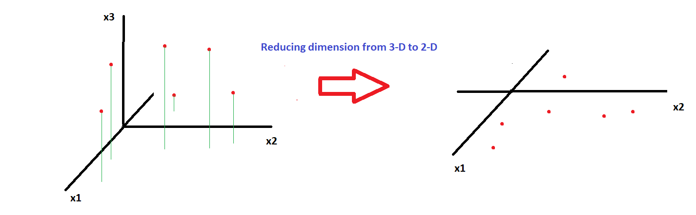
Principal Component Analysis (PCA) makes use of the same approach; however, in PCA, we find new coordinates which explain the maximum variation in the data. This is achieved by:
- first mean centring the data, i.e., making the mean of each column 0 and then
- finding the eigendecomposition of the covariance matrix(C) of the mean-centred variables. The eigendecomposition of a square matrix(covariance matrices are always square matrices) is given by:
C = V.Λ.VT
Here 'V' represents the matrix containing the eigenvectors (of covariance matrix C), which represent our new coordinates or principal components, and Λ is a diagonal matrix containing the eigenvalues of C.
Each diagonal value in Λ is an eigenvalue that represents the variance explained by the corresponding principal component. This procedure ensures that resulting new coordinates/features/principal components are designed to capture maximum variation in the data and are orthogonal (perpendicular) to each other (i.e., our new features are uncorrelated with each other).
The next step is where we choose the top few principal components (which explain the maximum variation successively) based on a pre-decided cut-off.
For example, if we have five features, to begin with, we will end up with five principal components as well, but we decide to keep only the first three as they explain 90% of the variation in the data. This effectively means that we have reduced the dimension of our feature space from 5 to 3 without losing much information.
In the next subsection, we look at an example of implementing PCA in trading.
Example of PCA in trading or investing with code in Python
Suppose Jim, a quant researcher working in a prop trading firm, is looking to develop a supervised ML model that predicts the direction of the overall market. He decides to use the past day returns of a basket of 7 tech stocks (assume they are the same stocks that were part of cluster 0 in the previous example) as features for the model.
To be more efficient with resources, Jim wants to reduce the dimensions of his feature space before he feeds the features to his supervised model.
What can help him here to quickly explore the possibility of reducing dimensions of data at hand?
Yes, you are right, it's PCA!
Below we showcase how Jim can go about conducting PCA using the scikit learn package in Python.
But first, we import the necessary libraries and fetch the data as follows:
['ADBE', 'CSCO', 'FB', 'GOOGL', 'INTC', 'MSFT', 'STLD']

Below, we plot the cumulative returns of the stocks to gauge the the performance as well as variation in the data:

The first step in PCA is to mean-centre the data. However, we will be using the PCA class from the scikit-learn library, which automatically scales the data (mean centres it), and so there is no need to do it manually (if you are using some other package, then you might have to do it yourself through matrix operation or using sklearn. preprocessing as done in the clustering example).
We will simply convert the data into a NumPy array format as required by the scikit learn library, import the PCA class and create an instance called 'model' to which we fit the raw data X:
PCA(n_components=7)
The hyperparameter of the model 'n_components' represents the dimension of the new co-ordinate/principal component space.
To begin with, we have initialized the model with the value of hyperparameter 'n_components' set to 7, which is the same as the number of original features in X(as we have 7 stocks).
We can access the principal component matrix/eigenvector matrix using the following command:
array([[ 0.43250364,  0.26595616,  0.43994419,  0.39167868,  0.39734818,
         0.37164424,  0.31502354],
       [ 0.31078208, -0.1784099 ,  0.31343949,  0.10492004, -0.16196493,
         0.17032255, -0.84088612],
       [ 0.07033748, -0.13062127,  0.35532243,  0.14605034, -0.83342892,
         0.01607169,  0.3681629 ],
       [-0.32754799, -0.62923875,  0.52613624,  0.06641712,  0.34086264,
        -0.30207809,  0.09001009],
       [ 0.23384309, -0.65419348, -0.5269365 ,  0.33600016,  0.0217246 ,
         0.32947421,  0.13328505],
       [-0.58953337,  0.22761183, -0.08110947,  0.7444334 , -0.0673928 ,
         0.05821513, -0.178753  ],
       [-0.44931934, -0.06824695,  0.14453582, -0.37783656, -0.00877099,
         0.79335935,  0.01753355]])
The principal components above have automatically been arranged in the order of the variance they explain(from high to low). So now, we can actually extract and plot the percentage of variance captured by each principal component as follows:
array([0.51, 0.21, 0.12, 0.06, 0.05, 0.03, 0.02])

Next, we visualize the cumulative variance explained:
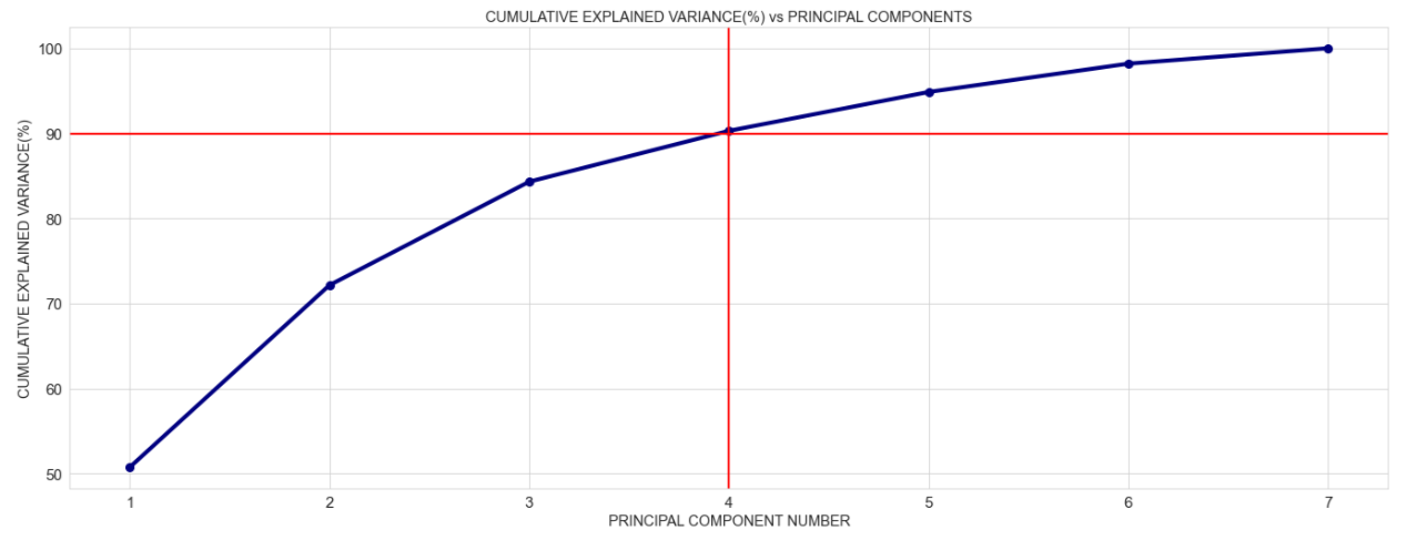
We can see above that the first 4 principal components explain almost 90% of the variance!
Which means that Jim can only use a PCA model with 4 principal components that is reduce the dimension from 7 to 4 at the cost of not explaining 10% variance in the data. Sounds like a good deal!
Below, we fit a new PCA model with 'n_components' = 4 and call it 'model_2':
We can now access the principal components and the percentage of variation explained by successive principal components:
array([[ 0.43250364,  0.26595616,  0.43994419,  0.39167868,  0.39734818,
         0.37164424,  0.31502354],
       [ 0.31078208, -0.1784099 ,  0.31343949,  0.10492004, -0.16196493,
         0.17032255, -0.84088612],
       [ 0.07033748, -0.13062127,  0.35532243,  0.14605034, -0.83342892,
         0.01607169,  0.3681629 ],
       [-0.32754799, -0.62923875,  0.52613624,  0.06641712,  0.34086264,
        -0.30207809,  0.09001009]])
array([0.5074455 , 0.21408255, 0.12162805, 0.05979477])
Finally, we can access our new features(Z), which correspond to the original data X projected in the principal component space:
array([[-1.12727573e-01, -6.67038416e-03, -1.48430796e-03,
         1.14035934e-03],
       [ 2.97074556e-02,  1.50265487e-02, -5.93081631e-02,
        -2.99243627e-02],
       [-5.47331714e-02, -4.75781399e-03, -1.65305232e-02,
         7.99569198e-03],
       ...,
       [-1.09056976e-02, -8.34552109e-05,  1.17423510e-02,
        -2.00353992e-03],
       [-4.17360862e-03,  2.44548028e-03,  1.19544647e-02,
         1.89425233e-02],
       [ 3.66918890e-02,  1.94108416e-02,  1.62907120e-02,
         4.10635097e-02]])
Let us look at the shape of original data and the dimension-reduced data:
(272, 7)
(272, 4)
Looking at the shapes of original data and the new reduced dimension data we can see how unsupervised learning algorithms like PCA can help us be more efficient with resources and to create new features to build parsimonious supervised models.
That is what Jim was looking for! He can now happily proceed to building his supervised model using these new features.
Other types of unsupervised algorithms
In the previous two sections, we have discussed two of the most popular types of of unsupervised algorithms namely clustering and dimensionality reduction algorithms. In addition to these, there are other types of unsupervised learning algorithms, which are used for specific purposes.
A useful implementation is latent variable modelling. Latent variables are variables that can't be directly observed but have an impact on some other observed variables.
Unsupervised learning can be used to understand the structure and patterns in the observed variables to model the latent variables. A good example of this is Hidden Markov Models, which can be used to detect the market regime in the context of financial markets.
Another common use case of unsupervised learning is in association rule learning. The aim here is to dig into large amounts of data and discover useful relations between features.
For example, supermarket firms can deploy this type of analysis to analyse customer baskets to see which items are likely to be bought together. The firm can place those items next to each other (for e.g., butter and cheese placed next to the bread section) to drive up the sales.
Challenges in unsupervised learning
Although we have seen how unsupervised learning can help us learn the patterns in our input data, it does come with its own challenges:
- As there is no label/target variable in unsupervised learning, there is no set way to calculate the performance of the model like we do in supervised learning algorithms.
- The user often has to spend considerable time interpreting the output. For example, the new features obtained from PCA need to be interpreted in the business context, and that itself takes time.
These are the reasons why unsupervised learning is often used in conjunction with supervised learning.
Conclusion
During the course of this blog, we saw how unsupervised learning algorithms provide us not only with insights into the input data but also new useful inputs for supervised machine learning algorithms as well.
We also discussed practical use cases for unsupervised learning in trading and investing with the help of two examples. You can learn all about in this course on unsupervised learning course.
As this was an introductory blog, we have only scratched the surface here. The scope of unsupervised learning is vast, and it encompasses applications implemented with the help of neural networks. Learn more about how neural network in trading can help enhance your skills.
Nonetheless, I hope that you have enjoyed reading this blog, and it has given you inspiration to look deeper into the realm of unsupervised learning and its applications in finance.
In case you're interested in Machine Learning and its applications in trading, you can't afford to miss this specialization on Machine Learning & Deep Learning in Financial Markets, where your will learn everything from simple logistic regression models to complex LSTM models. I hope this helps in your learning.
Till next time, happy learning!
Disclaimer: All investments and trading in the stock market involve risk. Any decisions to place trades in the financial markets, including trading in stock or options or other financial instruments is a personal decision that should only be made after thorough research, including a personal risk and financial assessment and the engagement of professional assistance to the extent you believe necessary. The trading strategies or related information mentioned in this article is for informational purposes only.