
This is the second installment of my series on regression analysis used in finance. In the first installment, we touched upon the most important technique in financial econometrics: regression analysis, specifically linear regression and two of its most popular flavours:
- univariate linear regression, and
- multivariate linear regression.
In this post, we apply our knowledge of regression to actual financial data. We will model the relationships from the previous post using Python and R. I run it in both (with downloadable code where applicable) so that readers fluent in one language or application can hopefully get more intuition on its implementation in others.
Many building blocks needed to develop and implement models are available as ready-to-wear software these days. Using them as-is is now standard practice among practitioners of quantitative trading.
Many assumptions underlie the linear regression model. Closely linked to them are also its shortcomings. If you plan to use linear regression for data analysis and forecasting, I'd recommend you look that up first. I intend to write on that topic next.
For now, I shall shrug those worries away and get on with the implementation.
Implementation using Python
There are many ways to perform regression analysis in Python. The statsmodels, sklearn, and scipy libraries are great options to work with.
For the sake of brevity, we implement simple and multiple linear regression using the first two.
I point to the differences in approach as we walk through the below code.
We use two ways to quantify the strength of the linear relationship between variables.
- Calculate pairwise correlations between the variables.
- Linear regression modeling (the preferred way).
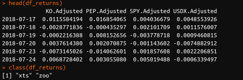
We start with the necessary imports and get the required financial data.
As discussed in my previous post, we work with the historical returns of Coca-Cola (NYSE: KO), its competitor PepsiCo (NASDAQ: PEP), the US Dollar index (ICE: DX) and the SPDR S&P 500 ETF (NYSEARCA: SPY).
We first create a scatter plot of the SPY and KO returns to better understand how they are related.
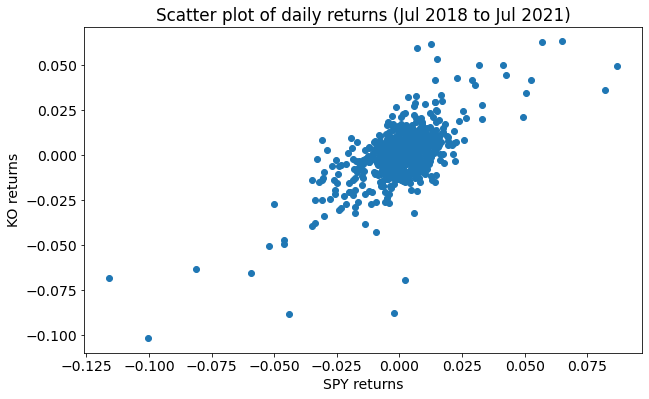
We also calculate correlations between different variables to analyze the strength of the linear relationships here.
| spy | ko | pep | usdx | |
|---|---|---|---|---|
| spy | 1.000000 | 0.684382 | 0.725681 | -0.045420 |
| ko | 0.684382 | 1.000000 | 0.738264 | -0.104387 |
| pep | 0.725681 | 0.738264 | 1.000000 | -0.011062 |
| usdx | -0.045420 | -0.104387 | -0.011062 | 1.000000 |
statsmodels
This library follows the classical approach in statistics to model building. It emphasizes statistical inference and hypothesis testing.
So we have nice features like a summary table (using the .summary routine). This style is similar to other statistical packages or languages like R or Stata.
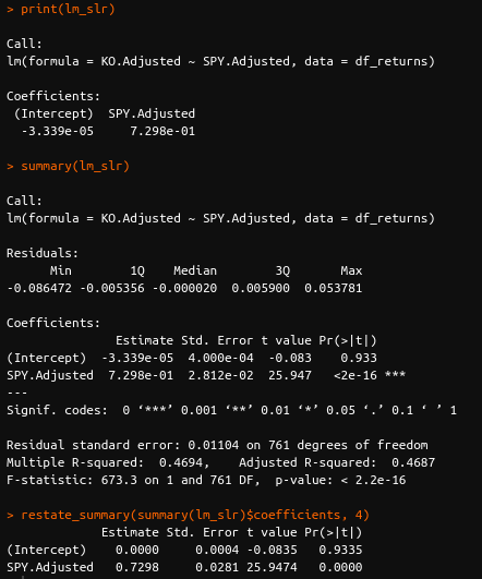
We then work with the SPY and the KO returns as the explanatory and response variables respectively, while implementing simple linear regression.
                          OLS Regression Results
==============================================================================
Dep. Variable:                     ko   R-squared:                       0.468
Model:                            OLS   Adj. R-squared:                  0.468
Method:                 Least Squares   F-statistic:                     655.5
Date:                Fri, 30 Jul 2021   Prob (F-statistic):          3.58e-104
Time:                        13:26:52   Log-Likelihood:                 2299.2
No. Observations:                 746   AIC:                            -4594.
Df Residuals:                     744   BIC:                            -4585.
Df Model:                           1
Covariance Type:            nonrobust
==============================================================================
                 coef    std err          t      P>|t|      [0.025      0.975]
------------------------------------------------------------------------------
Intercept  -5.622e-05      0.000     -0.138      0.890      -0.001       0.001
spy            0.7276      0.028     25.603      0.000       0.672       0.783
==============================================================================
Omnibus:                      194.805   Durbin-Watson:                   1.933
Prob(Omnibus):                  0.000   Jarque-Bera (JB):             2537.398
Skew:                          -0.785   Prob(JB):                         0.00
Kurtosis:                      11.898   Cond. No.                         69.8
==============================================================================

Notes:
[1] Standard Errors assume that the covariance matrix of the errors is correctly specified.
====================================================================
The intercept in the statsmodels regression model is -0.0001
The slope in the statsmodels regression model is 0.7276
====================================================================
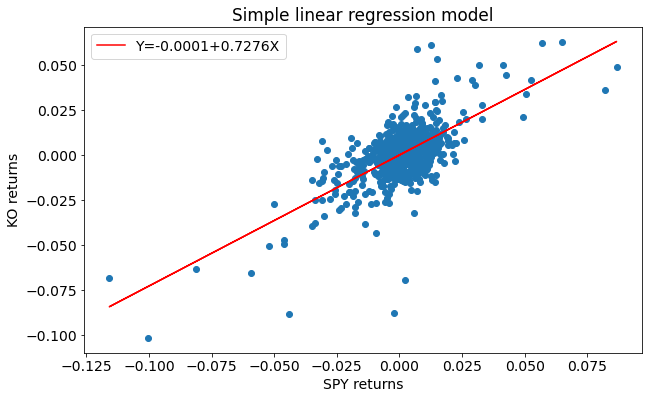
As per the results above, the model for KO's returns can be expressed as
\(Ŷ_𝑖\)= 0.0001+0.7276\(𝑋_𝑖\) (1)
The caret mark or ^ above the \(𝑌_𝑖\) indicates that it is the fitted (or predicted) value of KO's returns as opposed to the observed returns. We obtain it by computing the RHS of equation 1.
We plot the best fit line (i.e. the regression line) for the data set as shown below.

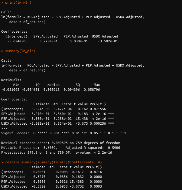
For multiple linear regression, we use SPY, PEP and DX returns as explanatory variables to explain KO returns.
                            OLS Regression Results
==============================================================================
Dep. Variable:                     ko   R-squared:                       0.599
Model:                            OLS   Adj. R-squared:                  0.597
Method:                 Least Squares   F-statistic:                     369.2
Date:                Fri, 30 Jul 2021   Prob (F-statistic):          1.12e-146
Time:                        13:28:51   Log-Likelihood:                 2404.2
No. Observations:                 746   AIC:                            -4800.
Df Residuals:                     742   BIC:                            -4782.
Df Model:                           3
Covariance Type:            nonrobust
==============================================================================
                 coef    std err          t      P>|t|      [0.025      0.975]
------------------------------------------------------------------------------
Intercept  -6.975e-05      0.000     -0.197      0.844      -0.001       0.001
spy            0.3267      0.036      9.080      0.000       0.256       0.397
pep            0.5016      0.033     15.212      0.000       0.437       0.566
usdx          -0.3510      0.096     -3.639      0.000      -0.540      -0.162
==============================================================================
Omnibus:                      167.282   Durbin-Watson:                   2.071
Prob(Omnibus):                  0.000   Jarque-Bera (JB):             4335.779
Skew:                          -0.310   Prob(JB):                         0.00
Kurtosis:                      14.794   Cond. No.                         273.
==============================================================================
Notes: [1] Standard Errors assume that the covariance matrix of the errors is correctly specified.
====================================================================
The intercept and slopes in the statsmodels regression model are


Intercept   -0.000070
spy          0.326696
pep          0.501565
usdx        -0.350995
dtype: float64
====================================================================
As per the results above, the model for KO's returns can be expressed as
\(Ŷ_𝑖\)=0.0+0.327\(𝑋_1,𝑖\)+0.502\(𝑋_2,𝑖\)−0.351\(𝑋_3,𝑖\) (2)
Similar to equation 1, the caret mark above the \(𝑌_𝑖\) indicates that it is the fitted (or predicted) value of KO's returns based on the historical returns on SPY, PEP, and USDX. We obtain it by computing the RHS of equation 2.
scikit-learn
We can also use the scikit-learn library for regressional analysis. However, it is geared to meet slightly different needs. The focus here is on the prediction/forecast of unobserved values.
Unlike statsmodels, here, we don't have the option of a full summary table with a detailed output.
Notice also how the features and output specified are done so in the .fit() routine (with features first and then the output variable). In statsmodels, we specified the parameters (in reverse order) when we instantiated the OLS class.
The coefficients obtained as you see here and in multiple regression, are the same with both libraries. That's what we'd expect to see, and fortunately, reality and expectations converge here.
The intercept in the sklearn regression result is -0.0001
The slope in the sklearn regression model is 0.7276
====================================================================
The intercept in the sklearn regression result is -0.0001
The slope in the sklearn regression model is 0.7276
====================================================================
The intercept in the sklearn regression result is -6.975208499046813e-05
The slope in the sklearn regression model is [ 0.32669603  0.50156517 -0.35099489]
Both approaches are good to know and conveniently use the same process (of instantiating a class, fitting the data onto the instance, and then using it for analysis or forecasting) as seen in the code snippets.
Our weapon of choice would be determined by what end goal we are trying to reach. To put it simply,
- if we are more interested in the analysis of historical data, we will choose the former, and
- if we want to predict the output when we feed new unseen data to the model, we will choose the latter
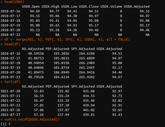
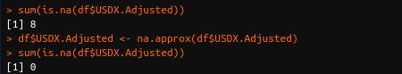
Implementation using R
We will now run the same operations as before.
I use RStudio as my IDE.
I reproduce below the relevant code snippets and their outputs.
The comments in the code will help us understand what happens at each stage.
Final thoughts
We've implemented linear regression using two different Python libraries and also in R. You might've noticed that there are slight differences in the coefficients computed. This is due to data differences when using the respective APIs.
I hope the implementation of linear regression on stock market data is clear to you now. In conclusion, I would say that regression analysis is a powerful tool in the quant finance trader's toolbox. It's far from perfect though, and operates under many assumptions which come along with limitations. In my next post, I will talk about them.
If you are interested in learning Machine Learning and its applications in trading, here's a highly-recommended track from Quantra - Learning Track: Machine Learning & Deep Learning in Financial Markets. It is perfect for beginners and experts, if you consider machine learning as an important part of the future in financial markets, you can't afford to miss this specialization.
Disclaimer: All investments and trading in the stock market involve risk. Any decisions to place trades in the financial markets, including trading in stock or options or other financial instruments is a personal decision that should only be made after thorough research, including a personal risk and financial assessment and the engagement of professional assistance to the extent you believe necessary. The trading strategies or related information mentioned in this article is for informational purposes only.
