
Hierarchical clustering is a powerful technique in the realm of data analysis and pattern recognition, offering a nuanced understanding of the relationships within datasets. This comprehensive guide delves into the intricacies of hierarchical clustering, specifically tailored for implementation in Python.
As the volume of raw data continues to increase rapidly, the prominence of unsupervised learning has grown. The primary objective of unsupervised learning is to unveil latent and intriguing patterns within unannotated datasets. Clustering stands out as the predominant algorithm in unsupervised learning, with applications spanning diverse domains, from medical diagnostics and facial recognition to stock market analysis. When clusters are used to form trading pairs or sector groupings, validating the resulting strategy requires rigorous backtesting, the course on backtesting trading strategies python shows you how to test cluster-derived strategies systematically, with proper out-of-sample evaluation. This blog specifically explores the intricacies of Hierarchical Clustering. You can learn all about in this course on unsupervised learning course.
By the end of this guide, readers will not only have a robust grasp of the theory behind hierarchical clustering but will also be equipped to apply this knowledge effectively using Python, ensuring a seamless integration of this powerful analytical tool into their data science toolkit.
This blog covers:
- What is hierarchical clustering?
- Example of hierarchical clustering
- Difference between clustering and classification
- Importance of K-Means in hierarchical clustering
- Difference between K-means clustering and hierarchical clustering
- Key concepts of hierarchical clustering
- Types of hierarchical clustering
- How to do hierarchical clustering in Python?
- Pros of hierarchical clustering in trading
- Cons of hierarchical clustering in trading
- Applications of hierarchical clustering
What is hierarchical clustering?
Hierarchical clustering is a technique in unsupervised machine learning that involves the organisation of data into a hierarchy of nested clusters. Unlike other clustering methods, hierarchical clustering creates a tree-like structure of clusters (dendrogram), which visually represents the relationships between data points.
- You can check out this introductory video on hierarchical clustering which is a free preview. This link will be accessible only after logging into the Quantra website.
- Further, you can enroll into our course on portfolio management using machine learning. In this course, starting from the video on “hierarchical clustering on stocks” in Section 8, unit 4 you shall get help with further learning about the implementation of hierarchical clustering in the trading domain.
Example of hierarchical clustering
In the realm of portfolio creation, envision a scenario where we seek to evaluate stock performance. Employing hierarchical clustering allows us to group akin stocks based on performance similarities, creating clusters grounded in shared financial traits like volatility, earnings growth, and price-to-earnings ratio.
Difference between clustering and classification
Both classification and clustering try to group the data points into one or more classes based on the similarity of various features. The difference lies in the way both works.
Classification is a supervised algorithm, where there are predefined labels (yi) assigned to each input data point (Xi).
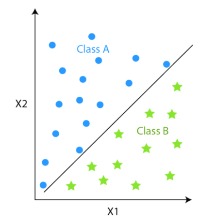
Whereas, clustering is an unsupervised algorithm where labels are missing meaning the dataset contains only input data points (Xi).
The other major difference is since classification techniques have labels, there is a need for training and test datasets to verify the model. In clustering, there are no labels so there is no need for training and test datasets.
Popular examples of classification algorithms are:
Examples of clustering algorithms are:
- Hierarchical clustering
- K-Means Clustering
- Mean Shift Clustering
- Spectral Clustering
Let us see the difference between hierarchical clustering and classification which is explained briefly in the table below.
|
Aspect |
Hierarchical Clustering |
Classification |
|
Objective |
Groups data points into hierarchical clusters |
Assign labels to data points |
|
Type of Learning |
Unsupervised learning |
Supervised learning |
|
Training Data |
No predefined classes; clusters based on similarity |
Requires labelled training data |
|
Output |
Dendrogram showing hierarchical cluster structure |
Predicted class labels for new data |
|
Algorithm Goal |
Discover inherent structures and relationships |
Learn patterns for accurate predictions |
|
Usage |
Exploratory data analysis; pattern discovery |
Predictive modelling; assigning labels |
|
Example |
Grouping stocks based on price movements |
Predicting stock trends as bullish/bearish |
In this article, we will deep dive into the details of only hierarchical clustering.
Importance of K-Means in Hierarchical Clustering
The answer to why we need Hierarchical clustering lies in the process of K-means clustering.
We will understand the K-means clustering in a layman's language.
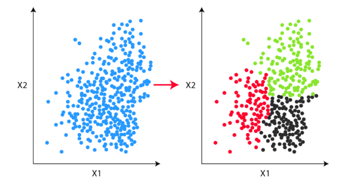
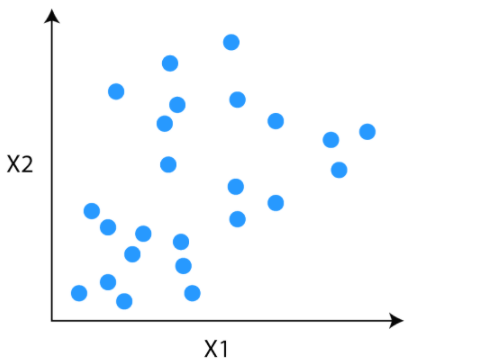
Consider this unlabeled data for our problem. Our task is to group the unlabeled data into clusters using K-means clustering.
Step 1
The first step is to decide the number of clusters (k). Let’s say we have decided to divide the data into two clusters.
Step 2
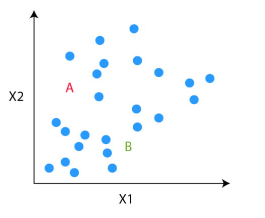
Once the clusters are decided, we randomly initialise two points, called the cluster centroids.
Step 3
In the third step, the algorithm goes to each of the data points and divides the points into respective classes, depending on whether it is closer to the red cluster centroid or green cluster centroid.
Step 4
In the fourth step, we move to the centroid step. We compute the mean of all the red points and move the red cluster centroid there and do the same for the green cluster centroid.
We will do steps 3 and 4 till the cluster centroid will not move any further. That is in this example, the colours of the point will not change any further.
The K-means process looks good, right?
Yes, but there is one problem or we can say the limitation of this process. At the beginning of the algorithm, we need to decide the number of clusters. But we don’t know how many clusters we need at the start.
Hierarchical clustering bridges this gap. In hierarchical clustering, we don’t need to define the number of clusters at the beginning.
Difference between K-means clustering and hierarchical clustering
Now, let us find out the difference between K-means clustering and hierarchical clustering. There is a thin line difference between the two and hence, it is important to find out the significant concepts that make each different from the other.
Below you can see the tabular representation of the same.
|
Aspect |
K-Means Clustering |
Hierarchical Clustering |
|
Objective |
Partition data into distinct clusters, where each cluster has similar data points. For instance, in trading, you might use K-means to group stocks based on similar volatility patterns. |
Group data into hierarchical clusters, forming a tree-like structure (dendrogram). For instance, hierarchical clustering could help create a hierarchy of stocks based on their correlation, indicating how closely related they are. |
|
The number of Clusters |
Predefined before clustering, and the algorithm aims to assign data points to the specified number of clusters. In trading, you might decide to group stocks into, say, three clusters based on specific criteria like price movements. |
Not predefined; the algorithm forms a dendrogram, allowing you to decide the number of clusters based on where you cut the tree. This flexibility can be useful when the optimal number of clusters is not known in advance. For instance, you might identify clusters of stocks with varying degrees of correlation. |
|
Computational Complexity |
Generally more computationally efficient as it assigns each data point to a single cluster. In trading, this could involve grouping stocks into clusters efficiently, making it easier to analyse and make investment decisions. |
Can be computationally intensive for large datasets, especially when forming the dendrogram. However, it offers a visual representation that can be valuable for understanding relationships among data points. For instance, you might use hierarchical clustering to create a visual representation of how different stocks are related in terms of price movements. |
|
Cluster Shape |
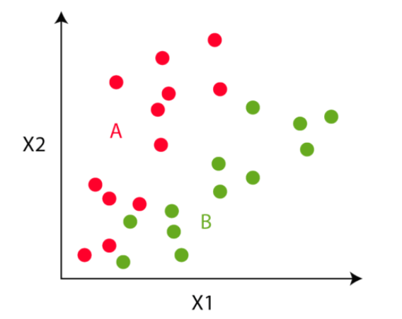
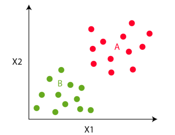
Assumes clusters are spherical, which may not be suitable for data with complex shapes. For example, if stocks have non-linear relationships, K-means might struggle to accurately capture them. |
Can handle clusters of various shapes, making it more adaptable to complex structures. In trading, where relationships between stocks can be intricate, hierarchical clustering might provide a more nuanced view of how stocks are grouped. |
|
Interpretability |
May lack interpretability for complex data, as it focuses on assigning points to clusters without explicitly showing relationships. For instance, K-means might group stocks based on volatility, but the underlying reasons for the grouping may not be immediately clear. |
Offers interpretability through the dendrogram, providing a visual representation of relationships among data points. This can be particularly beneficial in trading, where understanding how stocks are hierarchically grouped can inform investment strategies based on correlations. |
Key concepts of hierarchical clustering
Let us find the key concepts of hierarchical clustering before moving forward since these will help you with the in-depth learning of hierarchical clustering.
How to identify if two clusters are similar?
One of the ways to do so is to find the distance between clusters.
Measure of distance (similarity)
The distance between two clusters can be computed based on the length of the straight line drawn from one cluster to another. This is commonly known as the Euclidean distance.
The Euclidean distance between two points in either the plane or 3-dimensional space measures the length of a segment connecting the two points. It is the most obvious way of representing distance between two points.
If the (x1,y1) and (x2,y2) are points in 2-dimensional space then the euclidean distance between is:
(x2-x1)2 - (y2-y1)2
Other than Euclidean distance, several other metrics have been developed to measure distance such as:
- Hamming Distance
- Manhattan Distance (Taxicab or City Block)
- Minkowski Distance
The choice of distance metrics should be based on the field of study or the problem that you are trying to solve.
For example, if you are trying to measure the distance between objects on a uniform grid, like a chessboard or city blocks. Then Manhattan distance would be an apt choice.
Linkage Criterion
After selecting a distance metric, it is necessary to determine from where distance is computed. Some of the common linkage methods are:
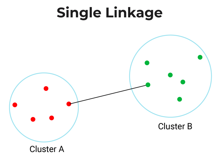
- Single-Linkage: Single linkage or nearest linkage is the shortest distance between a pair of observations in two clusters.
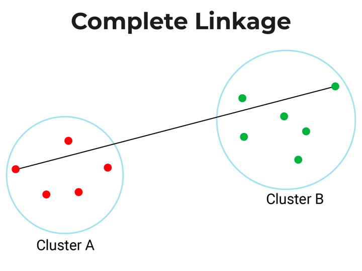
- Complete-linkage: Complete linkage or farthest linkage is the farthest distance between a pair of observations in two clusters.
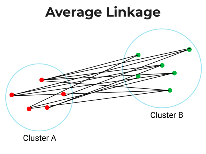
- Average-linkage: Average linkage is the distance between each observation in one cluster to every observation in the other cluster.
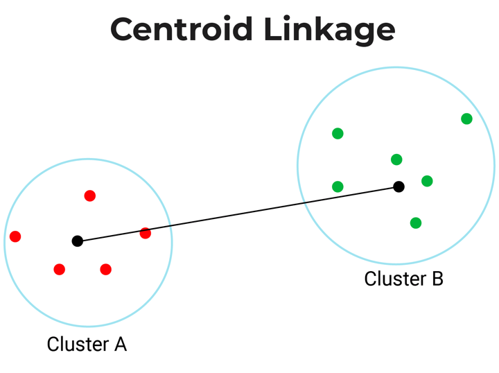
- Centroid-linkage: Centroid linkage is the distance between the centroids of two clusters. In this, you need to find the centroid of two clusters and then calculate the distance between them before merging.
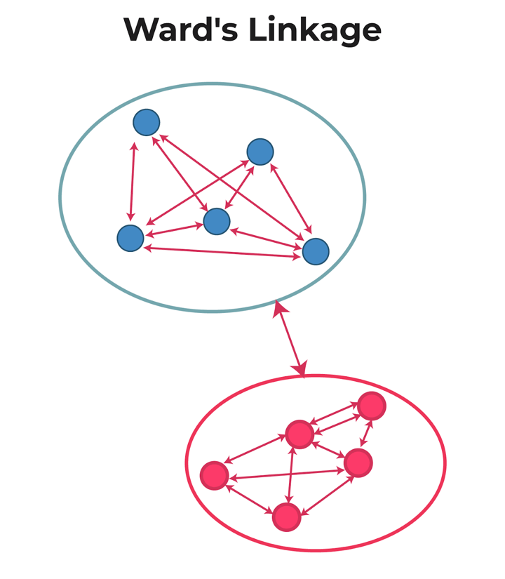
- Ward’s-linkage: Ward’s method or minimum variance method or Ward’s minimum variance clustering method calculates the distance between two clusters as the increase in the error sum of squares after merging two clusters into a single cluster.
In short, ward linkage is the distance which minimises variance in the cluster and maximises variance between the clusters.
The choice of linkage criterion is based on the domain application. Average-linkage and complete-linkage are the two most popular distance metrics in hierarchical clustering.
However, when there are no clear theoretical justifications for the choice of linkage criteria, Ward’s method is the default option.
How to choose the number of clusters?
To choose the number of clusters in hierarchical clustering, we make use of a concept called dendrogram.
What is a Dendrogram?
A dendrogram is a tree-like diagram that shows the hierarchical relationship between the observations. It contains the memory of hierarchical clustering algorithms.
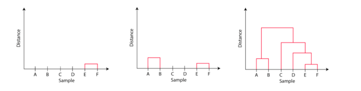
Just by looking at the Dendrogram, you can tell how the cluster is formed. Let's see how to form the dendrogram for the below data points.
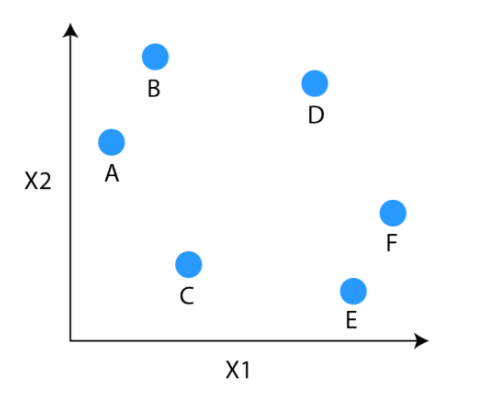
The observations E and F are closest to each other by any other points. So, they are combined into one cluster and also the height of the link that joins them together is the smallest. The next observations that are closest to each other are A and B which are combined together.
This can also be observed in the dendrogram as the height of the block between A and B is slightly bigger than E and F. Similarly, D can be merged into E and F clusters and then C can be combined to that. Finally, A and B combined to C, D, E and F to form a single cluster.
The important point to note while reading the dendrogram is that:
- The Height of the blocks represents the distance between clusters, and
- Distance between observations represents dissimilarities.
But the question still remains the same, how do we find the number of clusters using a dendrogram or where should we stop merging the clusters? Observations are allocated to clusters by drawing a horizontal line through the dendrogram.
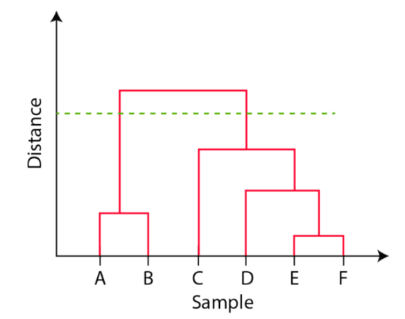
Generally, we cut the dendrogram in such a way that it cuts the tallest vertical line. In the above example, we have two clusters. One cluster has observations A and B, and a second cluster has C, D, E, and F.
Types of hierarchical clustering
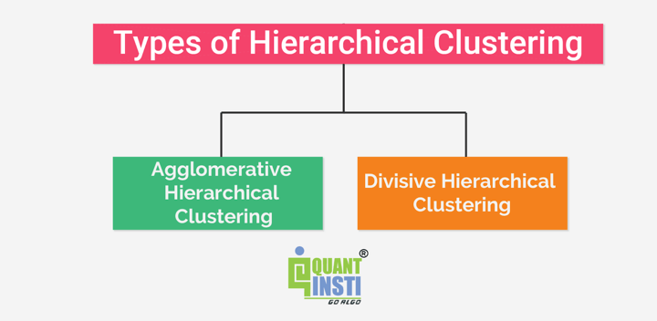
There are two types of hierarchical clustering:
- Agglomerative hierarchical clustering
- Divisive hierarchical clustering
Agglomerative Hierarchical Clustering
Agglomerative Hierarchical Clustering is the most common type of hierarchical clustering used to group objects in clusters based on their similarity. It's a bottom-up approach where each observation starts in its own cluster, and pairs of clusters are merged as one moves up the hierarchy.
Let us find out a few important subpoints in this type of clustering as shown below.
How does Agglomerative Hierarchical Clustering work?
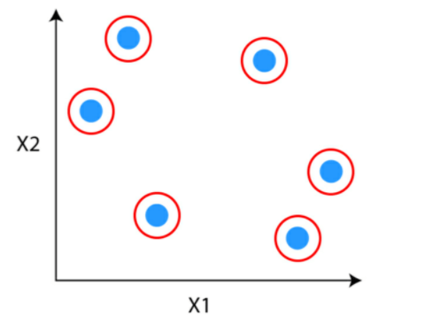
Suppose you have data points which you want to group in similar clusters.
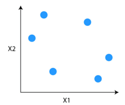
Step 1: The first step is to consider each data point to be a cluster.
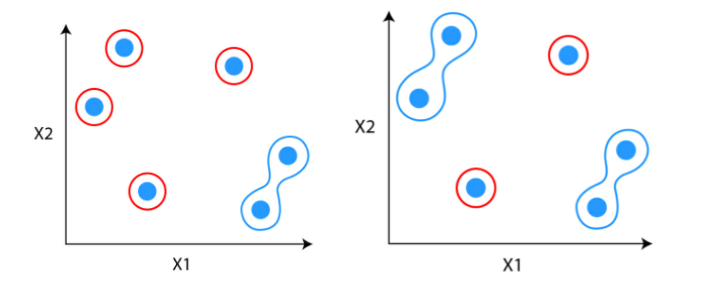
Step 2: Identify the two clusters that are similar and make them one cluster.
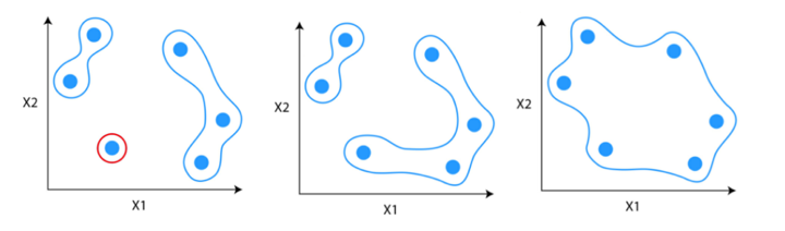
Step 3: Repeat the process until only single clusters remain
Divisive Hierarchical Clustering
Divisive hierarchical clustering is not used much in solving real-world problems. It works in the opposite way of agglomerative clustering. In this, we start with all the data points as a single cluster.
At each iteration, we separate the farthest points or clusters which are not similar until each data point is considered as an individual cluster. Here we are dividing the single clusters into n clusters, therefore the name divisive clustering.
Example of Divisive Hierarchical Clustering
In the context of trading, Divisive Hierarchical Clustering can be illustrated by starting with a cluster of all available stocks. As the algorithm progresses, it recursively divides this cluster into smaller subclusters based on dissimilarities in key financial indicators such as volatility, earnings growth, and price-to-earnings ratio. The process continues until individual stocks are isolated in distinct clusters, allowing traders to identify unique groups with similar financial characteristics for more targeted portfolio management.
How to do hierarchical clustering in Python?
To demonstrate the application of hierarchical clustering in Python, we will use the Iris dataset. The Iris dataset is one of the most common datasets that is used in machine learning for illustration purposes.
The Iris data has three types of Iris flowers which are three classes in the dependent variable. And it contains four independent variables which are sepal length, sepal width, petal length and petal width, all in cm. We will compare the original classes with the classes formed using hierarchical clustering methods.
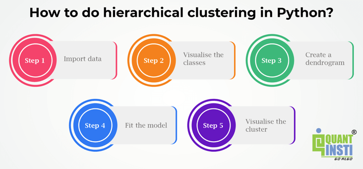
Let us take a look at the Python code with the steps below.
Step 1 - Import data
We will import the dataset from the sklearn library.
Output:
| sepal length (cm) | sepal width (cm) | petal length (cm) | petal width (cm) | flower_type | |
|---|---|---|---|---|---|
| 0 | 5.1 | 3.5 | 1.4 | 0.2 | 0 |
| 1 | 4.9 | 3.0 | 1.4 | 0.2 | 0 |
| 2 | 4.7 | 3.2 | 1.3 | 0.2 | 0 |
| 3 | 4.6 | 3.1 | 1.5 | 0.2 | 0 |
| 4 | 5.0 | 3.6 | 1.4 | 0.2 | 0 |
Step 2 - Visualise the classes
Output:
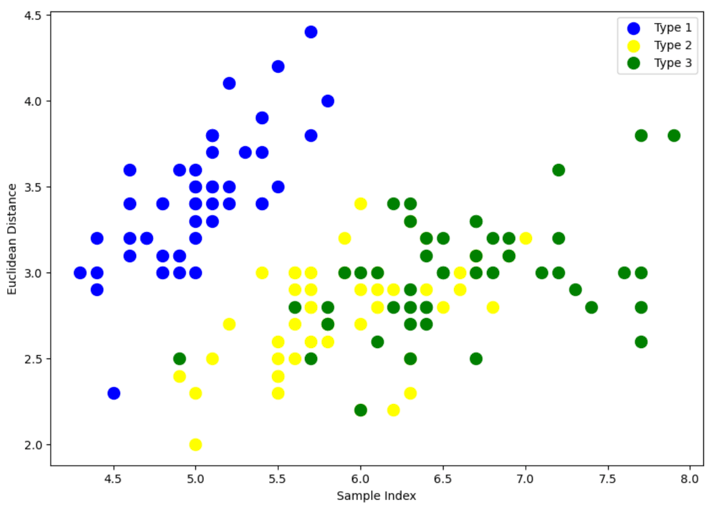
The above scatter plot shows that all three classes of Iris flowers overlap with each other. Our task is to form the cluster using hierarchical clustering and compare them with the original classes.
Step 3 - Create a dendrogram
We start by importing the library that will help to create dendrograms. The dendrogram helps to give a rough idea of the number of clusters.
Output:
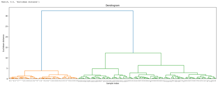
By looking at the above dendrogram, we divide the data into three clusters.
Step 4 - Fit the model
We instantiate AgglomerativeClustering. Pass Euclidean distance as the measure of the distance between points and ward linkage to calculate clusters' proximity. Then we fit the model on our data points. Finally, we return an array of integers where the values correspond to the distinct categories using lables_ property.
Output:
array([1, 1, 1, 1, 1, 1, 1, 1, 1, 1, 1, 1, 1, 1, 1, 1, 1, 1, 1, 1, 1, 1,
       1, 1, 1, 1, 1, 1, 1, 1, 1, 1, 1, 1, 1, 1, 1, 1, 1, 1, 1, 1, 1, 1,
       1, 1, 1, 1, 1, 1, 0, 0, 0, 0, 0, 0, 0, 0, 0, 0, 0, 0, 0, 0, 0, 0,
       0, 0, 0, 0, 0, 0, 0, 0, 0, 0, 0, 2, 0, 0, 0, 0, 0, 0, 0, 0, 0, 0,
       0, 0, 0, 0, 0, 0, 0, 0, 0, 0, 0, 0, 2, 0, 2, 2, 2, 2, 0, 2, 2, 2,
       2, 2, 2, 0, 0, 2, 2, 2, 2, 0, 2, 0, 2, 0, 2, 2, 0, 0, 2, 2, 2, 2,
       2, 0, 0, 2, 2, 2, 0, 2, 2, 2, 0, 2, 2, 2, 0, 2, 2, 0])
The above output shows the values of 0s, 1s, 2s, since we defined 4 clusters. 0 represents the points that belong to the first cluster and 1 represents points in the second cluster. Similarly, the third represents points in the third cluster.
Step 5 - Visualise the cluster
Output:
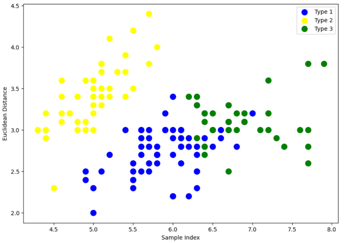
There is still an overlap between Type 1 and Type 3 clusters.
But if you compare with the original clusters in the Step 2 where we visualised the classes, the classification has improved quite a bit since the graph shows all three, i.e., Type 1, Type 2 and Type 3 not overlapping each other much.
Pros of hierarchical clustering in trading
Here are some pros of hierarchical clustering concerning trading.
- Diversification: By grouping similar assets, hierarchical clustering helps traders and investors identify opportunities for diversification within their portfolios. Diversification can mitigate risks associated with individual assets and enhance overall portfolio stability.
- Risk Management: Hierarchical clustering considers the relationships and correlations between assets, allowing for a more nuanced understanding of risk dynamics. This enables traders to allocate capital in a way that balances risk across different clusters, potentially leading to more effective risk management.
- Improved Decision-Making: By organising assets into clusters based on their inherent similarities, hierarchical clustering assists traders in making more informed decisions. It provides a structured framework for identifying opportunities, managing risks, and optimising portfolio allocations.
- Scalability: Hierarchical clustering can be applied to a wide range of assets and is scalable to different market conditions. Whether dealing with a small or large number of assets, the hierarchical approach remains applicable, making it versatile for various trading scenarios.
Cons of hierarchical clustering in trading
Let us now see some cons of hierarchical clustering that a trader can be aware of.
- Computational Complexity: Hierarchical clustering can be computationally intensive, especially as the number of assets increases. The process involves the calculation of distances between all pairs of assets, and the complexity can become a limitation for large datasets.
- Static Structure: The hierarchical structure formed by clustering is static once created. In dynamic markets, where correlations and relationships between assets change over time, the static nature of hierarchical clustering might not capture evolving market conditions.
- Subjectivity in Dendrogram Cutting: Determining the appropriate level to cut the dendrogram to form clusters can be subjective. Different cutting points may result in different cluster structures, leading to potential variations in portfolio outcomes.
- Assumption of Homogeneous Risk within Clusters: Hierarchical clustering assumes that assets within the same cluster share similar risk characteristics. However, this assumption may not always hold true, especially when assets within a cluster have diverse risk profiles.
- Limited to Historical Data: Hierarchical clustering relies on historical data for clustering decisions. If market conditions change significantly or unforeseen events occur, the historical relationships may not accurately reflect the current state of the market.
- Challenges with Noisy Data: In the presence of noisy or irrelevant data, hierarchical clustering may produce less meaningful clusters. Outliers or anomalies in the data can impact the accuracy of the clustering results.
Applications of hierarchical clustering
Hierarchical clustering finds applications in trading and finance, offering valuable insights and decision-making support across various areas:
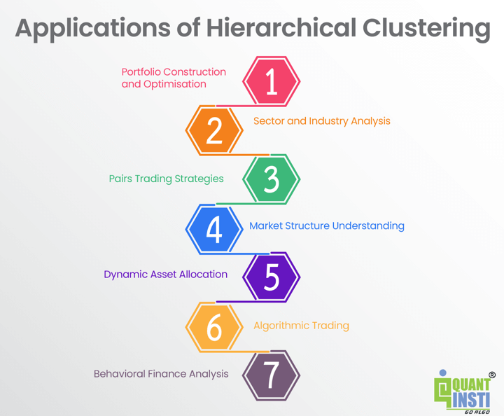
- Portfolio Construction and Optimisation: Hierarchical clustering aids in grouping assets with similar risk and return profiles, facilitating the construction of diversified portfolios. By optimising asset allocation within clusters, traders can achieve balanced portfolios that align with their risk tolerance and investment objectives.
- Sector and Industry Analysis: Hierarchical clustering can reveal natural groupings of assets related to specific sectors or industries. Traders can leverage this information for in-depth sector analysis, gaining insights into the dynamics and performance of different industry groups.
- Pairs Trading Strategies: Clustering helps identify pairs or groups of assets with strong correlations. Traders can implement pairs trading strategies by taking long and short positions in assets within the same cluster, aiming to profit from relative price movements.
- Market Structure Understanding: Clustering provides a visual representation of market structures through dendrograms. This aids traders in understanding relationships between assets and discerning overarching patterns and trends in the market.
- Dynamic Asset Allocation: The hierarchical structure allows for dynamic asset allocation strategies. As market conditions change, traders can adapt portfolios by updating the clustering structure, ensuring alignment with evolving market dynamics.
- Algorithmic Trading: Hierarchical clustering can be integrated into algorithmic trading strategies. Algorithms can use clustering results to make real-time decisions on portfolio rebalancing, trade execution, and risk management.
- Behavioral Finance Analysis: Clustering can help identify groups of assets exhibiting similar behavioural patterns. This information is valuable for understanding market sentiment, investor behaviour, and potential anomalies that can be exploited for trading opportunities.
Conclusion
This comprehensive guide on Hierarchical Clustering in Python equips readers with a deep understanding of the methodology's fundamentals and practical implementation. By exploring key concepts, such as agglomerative and divisive clustering, dendrogram interpretation, and Python implementation, readers gain the skills to apply hierarchical clustering to real-world datasets.
The pros and cons discussed highlight its relevance in trading, offering improved diversification, risk management, and decision-making. The outlined learning outcomes ensure readers can define the purpose, differentiate techniques, and proficiently apply hierarchical clustering, making this guide an essential resource for data analysts and traders seeking to enhance their analytical toolkit.
To explore more about hierarchical clustering, you can explore the course on Portfolio management using machine learning. With this course, you can learn to apply the hierarchical risk parity (HRP) approach on a group of 16 stocks and compare the performance with inverse volatility weighted portfolios (IVP), equal-weighted portfolios (EWP), and critical line algorithm (CLA) techniques.
Author: Updated by Chainika Thakar (Originally written by Vibhu Singh)
Note: The original post has been revamped on 8th January 2024 for accuracy, and recentness.
Disclaimer: All data and information provided in this article are for informational purposes only. QuantInsti® makes no representations as to accuracy, completeness, currentness, suitability, or validity of any information in this article and will not be liable for any errors, omissions, or delays in this information or any losses, injuries, or damages arising from its display or use. All information is provided on an as-is basis.
