By Tsotne Kutalia
Suppose you are an investor and you have a portfolio worth $1,000,000. While you are hoping your investment to grow, it is possible that in reality you incur a loss instead. How large can that loss be? What could be the approach to calculate the largest possible loss your portfolio may incur?
Furthermore, suppose that you work as a risk manager at a financial institution (e.g. bank, mutual fund or pension fund) which accrues deposits from people and invests them. In order to protect the depositors from excessive risk taken by the financial institution, a regulator authority demands them to report the largest possible loss (i.e. the largest risk they take) once in a certain period of time. How would you compute and report that greatest potential loss?
There is a way to tackle these problems. As you might have guessed, the best solution would be to have a single, computationally simple and easy-to-understand number which would answer all of the questions posed above. Value at Risk or simply VaR is a statistical measure which is computed based on a prespecified confidence level (i.e. the desired probability level) and it is interpreted as a threshold amount of loss which may be surpassed by actual loss incurred by a small prespecified probability. VaR has become an indispensable risk management tool in quant trading, providing a standardised and communicable measure of downside risk for both individual strategies and full portfolios. In other words, given the confidence level c (usually 90%, 95% or 99%), and L denoting the loss (as a random variable, i.e. any possible value of actual loss incurred), the VaR is a number such that
\( P(L > \text{VaR}) \leq 1 - c \)
(1)
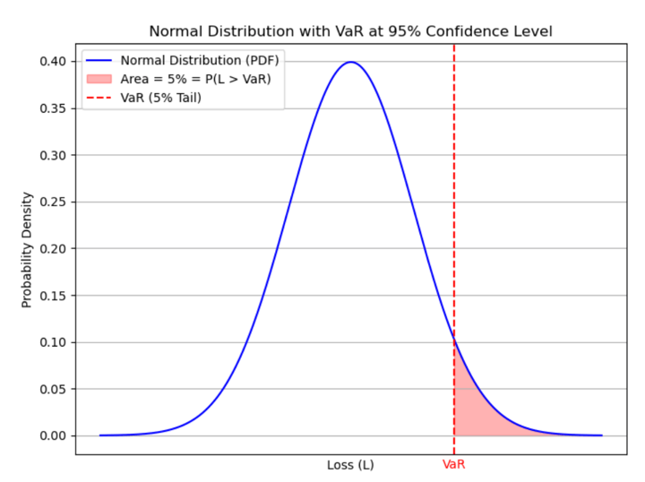
Note that here loss is taken as a positive number. Sometimes it is done the opposite way around. Negative gain can also be regarded as a loss. VaR is usually computed and reported for a short period of time, most likely on a daily basis.
Prerequisite knowledge needed to make most of this blog post:
- It is expected that you already understand concepts such as Random Variable, Standard Deviation, Covariance and Standard Normal Distribution.
- You are expected to know how to calculate Portfolio Variance.
- You have basic knowledge of using Python for trading, Python libraries and importing financial markets data.
This blog covers:
Computation of Portfolio VaR
Suppose you have a portfolio consisting of a certain number of assets and you have already computed the variance of the portfolio returns. Let us denote this quantity by σp2. Correspondingly, the standard deviation of a portfolio would also be computed and denoted by σp. Let z denote the value of a standard normal random variable corresponding to a certain confidence level c (let c = 0.95). For example, P(Z < z0.95) = 95%. In this case, z0.95 = 1.645. Finally, the portfolio value is denoted by W. The simplest way to compute the VaR corresponding to c confidence level would be as follows:
VaRp = z × σp × W
(2)
So, this quantity is measured in dollars and represents the largest amount that may be lost by c probability.
Example:
Given one-year monthly data of AMZN, TSLA, and AAPL within the time interval of 11/30/2023-11/29/2024, we construct a portfolio allocating $400,000 into AMZN, $300,000 into TSLA, and $300,000 into AAPL. So, in total, the portfolio is initially worth \( W = 1,000,000 \). We can define the weights vector as \( \mathbf{w} = \left[ 0.4, 0.3, 0.3 \right]^T \).
Then the returns of a given asset for a period of time \( t \) are computed by the formula:
\( R_t = \frac{R_t - R_{t-1}}{R_{t-1}} \)
(3)
As long as we have the returns for each asset, the portfolio return for a fixed period of time is computed by
\( R_p = \sum_{i=1}^{N} w_i R_i \)
(4)
which is merely the weighted sum of individual returns. Having \( R_p \) computed for all periods allows us to compute the standard deviation. Here we take a simple approach to compute the sample standard deviation directly from \( R_p \) by the formula:
\(s_p = \sqrt{\frac{(R_{\bar{p_i}} - \bar{R_p})^2}{n-1}} \)
(5)
In this example, we compute annual VaR, so since we are dealing with monthly data, in order to convert it to annualized standard deviation, we multiply \( s_p \times \sqrt{252} \).
There is another way of computing the portfolio standard deviation explained in. We can regard it as an estimate for \( σ_p \) in (2) (which is actually the true standard deviation of portfolio returns).
As long as we have computed the standard deviation, we need to first obtain the value of ( z = N-1 (0.95) = 1.645 ).
After which we compute the portfolio VaR (corresponding to 95% confidence level) by (2) which is:
\( \text{VaR}_p = 1.645 \times 0.2739 \times 1,000,000 = 450,597.66 \)
We interpret this quantity as the largest possible loss (by 95% confidence level) that can be incurred by the given portfolio. In other words, there is only 5% probability that the actual loss incurred will be larger than this amount.
Pros and Cons of using VaR as a risk measure
Value at Risk (VaR) is a widely used risk management tool that quantifies the potential loss in the value of a portfolio over a defined period for a given confidence interval. While it has advantages, it also has limitations. Here's a breakdown:
Pros of using VaR as a portfolio risk measure:
1. Simplicity and Intuition:
- VaR is relatively easy to understand and communicate. It provides a single number representing the worst expected loss over a specific time horizon at a given confidence level (e.g., 5% or 1%).
2. Standardised Metric:
- VaR is a standardised metric that allows for comparison across different portfolios, asset classes, or firms, making it useful for benchmarking risk.
3. Regulatory Acceptance:
- VaR is widely used in financial institutions and is required by regulators (e.g., Basel II and Basel III) for determining capital adequacy and managing risk exposure.
4. Useful for Risk Limits and Capital Allocation:
- VaR helps in setting risk limits, monitoring exposures, and determining the amount of capital to hold as a buffer against potential losses.
5. Quantitative Risk Measure:
- It provides a concrete, quantitative measure of risk that is useful in risk management, reporting, and decision-making.
Cons and Limitations of VaR:
1. No Information Beyond VaR:
- VaR tells you the threshold of potential loss but not how bad the loss can be beyond that threshold. For example, if a portfolio’s 1-day VaR is $1 million at a 95% confidence level, you don’t know how much the loss could be in the remaining 5% of the cases.
- This means that it doesn't account for "tail risk" or extreme events that may lead to larger losses. This brings us to yet another statistical risk measure called Expected Shortfall (ES), which fixes this problem to some extent.
2. Assumption of Normal Distribution:
- Many VaR models assume returns are normally distributed (or follow some other simple distribution), which can be unrealistic in practice, especially during times of market stress. Financial returns often exhibit "fat tails" (higher likelihood of extreme outcomes than normal distributions suggest).
3. Failure to Capture Liquidity Risk:
- VaR does not account for liquidity risk, which means it may underestimate the potential for loss in scenarios where assets are hard to sell quickly or in large volumes.
4. Time Horizon and Confidence Level Sensitivity:
- VaR depends on the chosen time horizon and confidence level, and its interpretation can vary significantly with these choices. A 1-day VaR at 95% confidence is very different from a 1-week VaR at 99% confidence.
- Changing the confidence level or time horizon can lead to vastly different risk assessments.
5. Does Not Capture Non-Linear Risks:
- VaR may fail to account for non-linear risks, especially for portfolios involving options or other derivatives. VaR assumes linear risk exposure, which can be inaccurate for portfolios with complex structures.
6. Limited to Historical Data:
- Since VaR is a statistical measure, it mostly relies on historical data to estimate the distribution of returns, and this past performance may not always be a reliable indicator of future risk, especially during periods of structural market changes or extreme events.
7. Can Encourage Risk-Taking:
- Since VaR only focuses on losses up to a certain threshold, it may encourage risk-taking behaviour beyond the VaR estimate, as losses that exceed the VaR are not directly visible within the risk measure.
8. Not an Effective Measure for Long-Term Risk:
- VaR is typically used for short-term risk assessments, and may not capture the risk of large drawdowns or adverse events that may unfold over longer time periods.
Conclusion
This blog illustrated the importance of VaR as a single, easily computable statistical measure of risk. We examined the process of computation of VaR and gave an example of deriving the result alongside its interpretation. While VaR provides a convenient and widely accepted measure of portfolio risk, it has several limitations, particularly in its inability to account for extreme events, non-linear risks, and liquidity concerns. It should ideally be used alongside other risk measures, such as stress testing, expected shortfall (ES), and scenario analysis, to gain a more comprehensive view of portfolio risk.
Files in the download:
- Excel file
The excel file illustrates the computation of Value at Risk for a portfolio consisting of three stocks. First, the asset returns are computed. Next, the portfolio returns are constructed based on a given weights vector. Finally, the Value at Risk is computed. - Python notebook
The python code snippets illustrate the computation of Value at Risk step by step. First, the code illustrates how to download the data of three stocks making up the portfolio. Then it constructs portfolio returns based on predefined weights allocated into each stock and finally, it computes the Value at Risk.
Bibliography:
- Jorion, P. (2001). Value At Risk: The new benchmark for managing Financial risk. New York: McGraw Hill.
Continue learning:
- Learn how to use Excel & Python to calculate various kinds of VaR.
- Compare VaR with Expected Shortfall to improve your risk management skills
- Learn quantitative portfolio management techniques such as Factor Investing, Risk Parity and Kelly Portfolio, and Modern Portfolio Theory.
- Learn, create and backtest various position sizing techniques such as Kelly, Optimal f, and volatility targeting on a trading strategy.
Note: The original post has been revamped on 17th Jan 2025 for recentness, and accuracy.
All investments and trading in the stock market involve risk. Any decision to place trades in the financial markets, including trading in stock or options or other financial instruments is a personal decision that should only be made after thorough research, including a personal risk and financial assessment and the engagement of professional assistance to the extent you believe necessary. The trading strategies or related information mentioned in this article is for informational purposes only.