
The Central Limit Theorem (CLT) is often referred to as one of the most important theorems, not only in statistics but also in the sciences as a whole. In this blog, we will try to understand the essence of the Central Limit Theorem with simulations in Python.
Contents
- Samples and the Sampling Distribution
- What is the Central Limit Theorem?
- Central Limit Theorem - Statement & Assumptions
- Demonstration of CLT in action using simulations in Python with example
- Example 1 - Exponentially distributed population
- Example 2 - Binomially distributed population
- An Application of CLT in Investing/Trading
- The Challenge for Investors
- The Great Assumption of Normality in Finance
- The Shapiro-Wilk test
- The Role of Central Limit Theorem
- Testing Normality of Weekly and Monthly Returns
- Confidence Intervals
Samples and the Sampling Distribution
Before we get to the theorem itself, it is first essential to understand the building blocks and the context. The main goal of inferential statistics is to draw inferences about a given population, using only its subset, which is called the sample.
We do so because generally, the parameters which define the distribution of the population, such as the population mean \(\mu\) and the population variance \(\sigma^{2}\), are not known.In such situations, a sample is typically collected in a random fashion, and the information gathered from it is then used to derive estimates for the entire population.
The above-mentioned approach is both time-efficient and cost-effective for the organization/firm/researcher conducting the analysis. It is important that the sample is a good representation of the population, in order to generalize the inferences drawn from the sample to the population in any meaningful way.
The challenge though is that being a subset, the sample estimates are well, just estimates, and hence prone to error! That is, they may not reflect the population accurately.
For example, if we are trying to estimate the population mean \((\mu)\) using a sample mean \((\bar x)\), then depending on which observations land in the sample, we might get different estimates of the population with varying levels of errors.What is the Central Limit Theorem?
The core point here is that the sample mean itself is a random variable, which is dependent on the sample observations.
Like any other random variable in statistics, the sample mean \((\bar x)\) also has a probability distribution, which shows the probability densities for different values of the sample mean.This distribution is often referred to as the 'sampling distribution'. The following diagram summarizes this point visually:
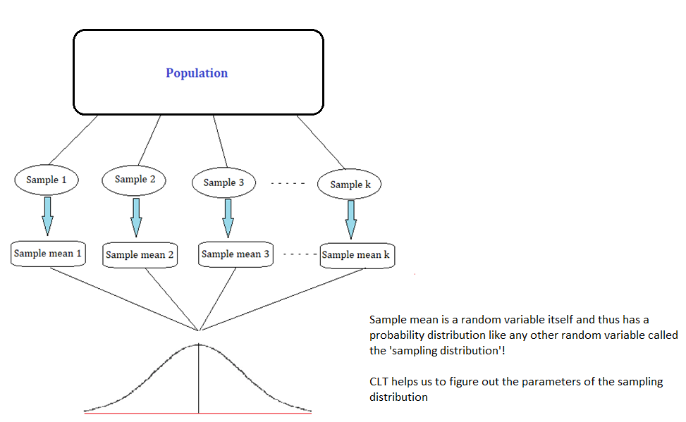
The Central Limit Theorem essentially is a statement about the nature of the sampling distribution of the sample mean under some specific condition, which we will discuss in the next section.
Central Limit Theorem - Statement & Assumptions
Suppose \(X\) is a random variable(not necessarily normal) representing the population data. And, the distribution of \(X\), has a mean of \(\mu\) and standard deviation \(\sigma\). Suppose we are taking repeated samples of size 'n' from the above population.Then, the Central Limit Theorem states that given a high enough sample size, the following properties hold true:
- Sampling distribution's mean = Population mean \((\mu)\), and
- Sampling distribution's standard deviation (standard error) = \(\sigma/√n\), such that
- for n ≥ 30, the sampling distribution tends to a normal distribution for all practical purposes.
In other words, for a large n, $$\bar{x}\longrightarrow\mathbb{N}\left(\mu,\frac{\sigma}{\sqrt{n}}\right)$$
In the next section, we will try to understand the workings of the CLT with the help of simulations in Python.
Demonstration of CLT in action using simulations in Python with examples
The main point demonstrated in this section will be that for a population following any distribution, the sampling distribution (sample mean's distribution) will tend to be normally distributed for large enough sample size.
We will consider two examples and check whether the CLT holds.
- Example 1 - Exponentially distributed population
- Example 2 - Binomially distributed population
Example 1 - Exponentially distributed population
Suppose we are dealing with a population which is exponentially distributed. Exponential distribution is a continuous distribution that is often used to model the expected time one needs to wait before the occurrence of an event.
The main parameter of exponential distribution is the 'rate' parameter \(\lambda\), such that both the mean and the standard deviation of the distribution are given by \((1/\lambda)\).The following represents our exponentially distributed population:

f(x) = \(\cases{\lambda e^{-\lambda x} & if x> 0\cr0 & \text{otherwise}}\)
E(X) = \(1/\lambda\) = \(\mu\)V(X) = \(1/\lambda^2\) = \(\sigma^2\), which means SD(X) = \(1/\lambda\) = \(\sigma\)
We can see that the distribution of our population is far from normal! In the following code, assuming that \(\lambda\)=0.25, we calculate the mean and the standard deviation of the population:
Population mean: 4.0
Population standard deviation: 4.0
Now we want to see how the sampling distribution looks for this population. We will consider two cases, i.e. with a small sample size (n= 2), and a large sample size (n=500).
First, we will draw 50 random samples from our population of size 2 each. The code to do the same in Python is given below:
For each of the 50 samples, we can calculate the sample mean and plot its distribution as follows:

We can observe that even for a small sample size such as 2, the distribution of sample means looks very different from that of the exponential population, and looks more like a poor approximation of a normal distribution, with some positive skew.
In case 2, we will repeat the above process, but with a much larger sample size (n=500):

The sampling distribution looks much more like a normal distribution now as we have sampled with a much larger sample size (n=500).
Let us now check the mean and the standard deviation of the 50 sample means:
| Sample means | |
|---|---|
| sample 1 | 4.061534 |
| sample 2 | 4.052322 |
| sample 3 | 3.823000 |
| sample 4 | 4.261559 |
| sample 5 | 3.838798 |
We can observe that the mean of all the sample means is quite close to the population mean \((\mu = 4)\).
Similarly, we can observe that the standard deviation of the 50 sample means is quite close to the value stated by the CLT, i.e., \((\sigma/ \sqrt{n})\) = 0.178.
0.18886796530269118
0.17888543819998318
Thus, we observe that the mean of all sample means is very close in value to the population mean itself.
Also, we can observe that as we increased the sample size from 2 to 500, the distribution of sample means increasingly starts resembling a normal distribution, with mean given by the population mean \(\mu\) and the standard deviation given by \((\sigma / \sqrt{n})\) , as stated by the Central Limit Theorem.Example 2 - Binomially distributed population
In the previous example, we knew that the population is exponentially distributed with parameter \(\lambda\)=0.25.Now you might wonder what would happen to the sampling distribution if we had a population which followed some other distribution say, Binomial distribution for example.
Would the sampling distribution still resemble the normal distribution for large sample sizes as stated by the CLT?
Let's test it out. The following represents our Binomially distributed population (recall that Binomial is a discrete distribution and hence we produce the probability mass function below):
where, \(0\leq p\leq 1\)
E(X) = kp = \(\mu\)
V(X) = kp(1-p), which means SD(X) = \(\sqrt{kp(1-p)}\) = \(\sigma\)
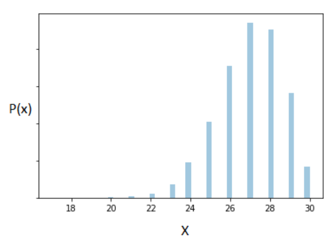
As before, we follow a similar approach and plot the sampling distribution obtained with a large sample size (n = 500) for a Binomially distributed variable with parameters k=30 and p = 0.9

For this example, as we assumed that our population follows a Binomial distribution with parameters k = 30 and p =0.9
Which means if CLT were to hold, the sampling distribution should be approximately normal with mean = population mean = \(\mu= 27\) and standard deviation = \(\sigma/\sqrt{n}\) = 0.0734.26.99175999999999
0.06752975459086173
And the CLT holds again, as can be seen in the above plot.
The sampling distribution for a Binomially distributed population also tends to a normal distribution with mean \(\mu=\) and standard deviation \(\sigma/\sqrt{n}\) for large sample size.An Application of CLT in Investing/Trading
The Challenge for Investors
A common challenge that an investor faces is to determine whether a stock is likely to meet her investing goals. For example, consider Jyoti, who is looking to invest in a safe stock for the next five years.
Being a risk averse investor, she would only feel comfortable to invest in a stock if it gives preferably non-negative monthly returns on average and where she can be reasonably confident that her average monthly return will not be less than -0.5%.
Jyoti is very interested in the ITC (NSE: ITC) stock, but wants to make sure that it meets her criterion. In such a case, is there some theoretical/statistical framework which can help her to reach a conclusion about the average monthly return of the ITC stock with some confidence?
The answer is yes! And such a statistical framework is based on the assumption of the return distribution, which in turn is based on the Central Limit Theorem (CLT).
In the next section, we start conducting our analysis on the ITC stock data.
The Great Assumption of Normality in Finance
In finance models (like the Black-Scholes option pricing model), we usually assume that the price series is log-normally distributed, and so returns are normally distributed.
And so for investors and traders, who use these models to invest or trade in the market, a lot depends on whether or not the assumption of normality actually holds in the markets.
Let us check it out for the ITC (NSE: ITC) stock in which Jyoti is interested. To conduct the analysis, we first import some standard Python libraries and fetch the daily Close-Close ITC stock data from the yfinance library.
We then do a visual analysis of the distribution of daily returns. Below is the code for the same:
| Date | Adj Close | daily_return |
|---|---|---|
| 2010-01-05 | 67.7443 | 0.009807 |
| 2010-01-06 | 67.9030 | 0.002340 |
| 2010-01-07 | 67.6914 | -0.003121 |
| 2010-01-08 | 67.8369 | 0.002147 |
| 2010-01-11 | 67.8633 | 0.000389 |
Now that we have the daily log returns for ITC, in the diagrams below we visualize both the returns and their distribution:
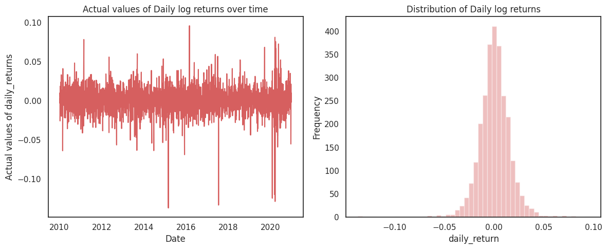
We can observe that in the ten years we are using, the daily return for ITC is centred around 0. However, there have been multiple occasions when it has breached the five percent mark on the upside and even a negative ten percent mark on the downside.
This is what is responsible for the higher kurtosis or the fat-tails which is not the case with a normal distribution. The plot of the distribution of daily returns also looks leptokurtik.
However, our conclusions are based on visual analysis up till now. To validate them, we need to conduct a proper statistical test to check the normality/non-normality of the data, which is what we do in the next section.
The Shapiro-Wilk test
We can conduct a statistical test, the Shapiro-Wilk test, to check for normality of data. It is the most powerful test when testing for a normal distribution.
If the p-value is larger than 0.01, and we assume a normal distribution with 99% confidence, else we reject the null hypothesis of normality.
We run the above mentioned test below on the daily log returns using the shapiro function from the scipy library:
The p-value is 5.638797613287179e-35, hence we reject that the data is normally distributed with 99% confidence
The p-value is 5.638797613287179e-35, hence we reject that the data is normally distributed with 99% confidence.
Thus, we have statistically shown that the assumption of normality does not hold for the daily level log returns. This puts into question the use and relevance of the most popular and beloved normal distribution!
Is there any hope?
Is there some theoretical grounding that can justify the use of Normal distribution in Finance?
The answer emanates from the Central Limit Theorem itself, as we will discuss in the next section.
The Role of Central Limit Theorem
Recall from the previous blog what the CLT actually states. Suppose \(X\) is a random variable (not necessarily normal) representing the population data. And, the distribution of \(X\), has a mean of \(μ\) and standard deviation \(σ\). Suppose we are taking repeated samples of size 'n' from the above population.Then for a high enough sample size 'n', the the following properties hold true:$$\bar{x}\longrightarrow\mathbb{N}\left(\mu,\frac{\sigma}{\sqrt{n}}\right)$$But we know that, $$\bar{x} = \left[\frac{x_1+x_2 +x_3+\ldots +x_n}{n}\right]$$which means, $$\left[\frac{x_1+x_2 +x_3+\ldots +x_n}{n}\right]\longrightarrow\mathbb{N}\left(\mu,\frac{\sigma}{\sqrt{n}}\right)$$which is same as, $$\left[{x_1+x_2 +x_3+\ldots +x_n}\right]\longrightarrow\mathbb{N}\left(n\mu,\sigma{\sqrt{n}}\right)$$Thus, we have shown that according to the Central Limit Theorem, if \([x_1, x_2, x_3, \ldots,x_n]\) is a random sample of size n from a population of any distribution, then the sum of \([x_1, x_2, x_3, \ldots,x_n]\) i.e. \([x_1 + x_2 + x_3+ \ldots+x_n]\) is also Normally distributed, given 'n' is large.In our case, the repeated random samples are nothing but consecutive daily log returns of the stock. As the log returns are additive in nature, if we sample daily log returns for each day of the week (assuming there are five trading days in the week), and sum them up, we get the weekly return.
Similarly, if we add up the daily log returns of all the trading days in a month we get the monthly return.
Testing Normality of Weekly and Monthly Returns
One of the major aspects when building quantitative finance models based on stock returns is that there exists a population data generating process, that is generating the observed data, and we are sampling from that data.
For example, we assume that there exists a data generating process which is generating stock returns. The parameters which define the distribution of this process are not known, but need to be estimated.
If we use daily log returns, we are sampling the data at the end of each trading day from previous close price. Thus, \({x_1}\) is the log return at the end of first trading day, \({x_2}\) is the log return at the end of second trading day and so on. Now if we sample for 'n' days, we have a sample of size 'n'. We have already seen that the daily log returns are not normally distributed.Let us see what happens when we analyse weekly returns instead of daily returns (i.e. we increase n from 1 to 5).
As the log returns are additive in nature, if we sample daily log returns for each day of the week(assuming there are five trading days in the week), the weekly return is given by \([x_1 + x_2 + x_3+ x_4 +x_5]\).In the following, we plot the weekly returns and their distribution for weekly log returns for the ITC stock:
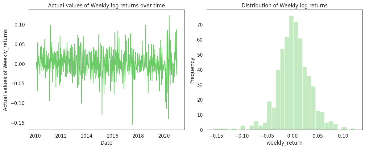
To check if the weekly returns are Normally distributed or not we again conduct the Shapiro-Wilk normality test on weekly data:
The p-value is 6.851103240279599e-09, hence we reject that the data is normally distributed with 99% confidence
A small p-value indicates that even when we sample at a weekly level, the data is not normal. Now, we further we analyse monthly returns (i.e. increase sample size to 20) and check if the monthly returns are normally distributed.
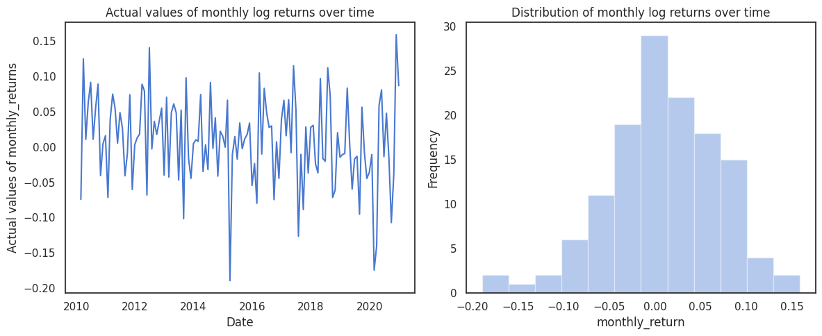
The p-value is 0.2705831527709961, hence we can assume that the data is normally distributed with 99% confidence
The p-value for the Shapiro-Wilk test for monthly data is quite large, which leads to the conclusion that the monthly returns are normally distributed with 99% confidence!
We summarize our analysis in the table below:

Thus, we can see that although daily and weekly frequency return data can't be assumed to be normally distributed, monthly data can be safely assumed to be normally distributed with 99% confidence, in line with the Central Limit Theorem.
Confidence Intervals
Coming back to Jyoti's investment problem, as we can safely assume monthly returns to be normally distributed, we can utilize the statistical concept of confidence intervals for getting a range for average monthly return with some confidence.
In general, under the assumption of normality, the confidence interval is given by:
$$ \bar{x} \pm z* \frac{s}{\sqrt{n}}$$, where, z is the z-score associated with a particular confidence level.So if we want to get the 95% confidence interval for the average monthly return, as almost 95% of the data for a standard normal variate lies between roughly +/- 2 standard deviations, the z-score would be 2 (1.96 to be precise!).
Also, as we do not know the population standard deviation \(σ\), we will use the sample standard deviation \(s\) in its place.In the code below, we calculate the confidence interval for average monthly return:
Thus, we see that although the point estimate for average monthly return for ITC stock is 0.868%.
However, the range estimate is (-0.2,1.9), i.e., we can be 95% confident that the average monthly return will not be below -0.2%.
This provides a solid theoretical argument for Jyoti to invest in this stock as it meets her criteria.
Conclusion
Earlier in this blog, we demonstrated with the help of two examples that irrespective of the shape of the original population distribution, the sampling distribution will tend to a normal distribution as stated by the CLT.
In these examples, we knew all the parameters of our populations. However, even if we did not know the population parameters, we can reverse engineer the estimates for the population parameters assuming that the sampling distribution is normally distributed. Therein lie the importance and appeal of the Central Limit Theorem.
Later on, we saw how the Central Limit Theorem (CLT) provides the basis for the very useful and widely used concept of confidence intervals, which can help investors and traders to make important decisions.
The point to keep in mind is that confidence intervals are probabilistic, and although even when we are 95% confident, there is still a 5% chance of things not happening the way we want.
However, as they say: "all models are wrong, but some are useful", and that is what we look to make use of!
In addition to confidence intervals, many important techniques which are used frequently in statistics and research, such as hypothesis testing, also emanate and rely on the Central Limit Theorem.
Thus, it would not be wrong to say that the CLT forms the backbone of inferential statistics in many ways and has rightly earned its place as one of the most consequential theorems in all of the sciences!
I hope you have enjoyed reading this blog. Do share your comments below. Till the next time, keep learning!
Disclaimer: All investments and trading in the stock market involve risk. Any decisions to place trades in the financial markets, including trading in stock or options or other financial instruments is a personal decision that should only be made after thorough research, including a personal risk and financial assessment and the engagement of professional assistance to the extent you believe necessary. The trading strategies or related information mentioned in this article is for informational purposes only.
