
When analysing the performance of financial securities, we give a lot of importance to the mean and the standard deviation as measures of the average return and risk, respectively.
However, the risk-adjusted performance of financial securities also depends upon the risks which arise due to the shape of the distribution of their returns. These are the higher-moment risks such as the skewness and kurtosis risks, which need to be taken into consideration for proper evaluation.
In this blog, we discuss the concept of kurtosis and its application in understanding the risk profiles of financial securities. In addition, we also glance over some common misconceptions regarding the calculation and interpretation of kurtosis.
Contents
- What is kurtosis?
- Excess kurtosis
- Classification of distributions based on kurtosis
- Kurtosis-risk/ tail-risk in financial securities
- A common error in interpretation of kurtosis
- Analysing the tail risk in S&P 500 and Bitcoin
- Conclusion
What is kurtosis?
Kurtosis is a statistical measure which quantifies the degree to which a distribution of a random variable is likely to produce extreme values or outliers relative to a normal distribution.
From extreme values and outliers, we mean observations that cluster at the tails of the probability distribution of a random variable. In other words, kurtosis measures the 'tailedness' of distribution relative to a normal distribution.
Along with variance and skewness, which measure the dispersion and symmetry, respectively, kurtosis helps us to describe the 'shape' of the distribution.
Mathematically, the kurtosis of a distribution of a random variable X, with a mean μ and standard deviation σ is defined as the ratio of the fourth moment to the square of the variance \(σ^2\)
ie. \( kurtosis = \frac{\text{The fourth moment}}{σ^{4}} = \frac{\frac{\sum \limits _{j=1} ^{n} (X_{j}-μ)^{4}}{n}}{σ^{4}} \)
From the above expression, we can already see that outliers will significantly impact this value.
This is because for any outlier \(x_p\) the value \((x_p- μ)\) will tend to be large anyway, but then the outliers contribution to the sum is raised to the power of four
i.e. \((x_p-μ)^4\)
In other words, the key factor that would determine the value of kurtosis is the number and size of the outliers/extreme values, which are reflected in heavier/fatter tails of the distribution.
Contrary to popular perception, kurtosis does not measure the peakedness of the distribution, and the only unambiguous interpretation of kurtosis is with regard to the heaviness or lightness of tails of the distribution, relative to a normal distribution (we will see an example of this in a subsequent section).
Excess kurtosis
There exists one more method of calculating the kurtosis called 'excess kurtosis'. As kurtosis is calculated relative to the normal distribution, which has a kurtosis value of 3, it is often easier to analyse in terms of excess kurtosis.
As the name suggests, it is the kurtosis value in excess of the kurtosis value of the normal distribution. This means that for a normal distribution with any mean and variance, the excess kurtosis is always 0.
$$ Excess\ kurtosis = \frac{\text{The fourth moment}}{σ^{4}} - 3 = \frac{\frac{\sum \limits _{j=1} ^{n} (X_{j}-μ)^{4}}{n}}{σ^{4}} - 3 $$
Many resources refer to 'excess kurtosis' as 'kurtosis' and hence to avoid any confusion one must clarify this point beforehand.
In the next section, we will learn about the three categories of distributions based on the kurtosis.
Classification of distributions based on kurtosis/excess kurtosis
Any statistical distribution can be categorised into one of the three categories based on its kurtosis/excess kurtosis:
Mesokurtic
When the kurtosis of distribution is 3, i.e. the excess kurtosis is equal to 0, the distribution is called mesokurtic. This means the distribution is a normal distribution. ('meso' stands for medium or middle). As the kurtosis of a mesokurtic distribution is neither positive nor negative, it serves as a baseline for the two other categories.
Platykurtic
The second category is that of platykurtic distributions which have negative excess kurtosis values. Negative values of excess kurtosis indicate that distribution has short/thin tails. A good example of such a distribution is the continuous uniform distribution.
Leptokurtic
The last category is that of leptokurtic distributions which have positive excess kurtosis. A large positive kurtosis indicates a distribution where more of the values are located away from the mean i.e. in the tails of the distribution. Thus, leptokurtic distributions are characterized by fatter tails. A good example is the Laplace distribution.
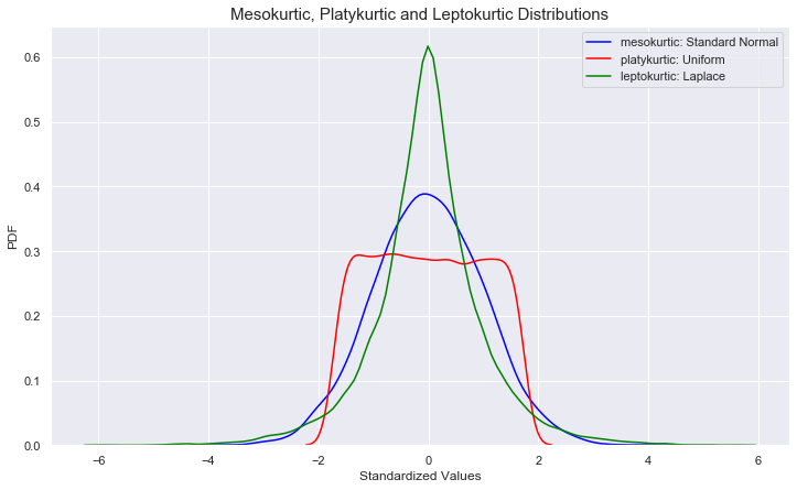
In the following Python code, we draw random samples from three example distributions with roughly equal mean, equal variance and which are almost symmetrically distributed around their means. (New to Python? Get started with our Python for trading course for better understanding.)
These distributions are:
- Standard Normal (mesokurtic)
- Uniform (platykurtic)
- Laplace (leptokurtic)
Now let us summarize the information about the means, standard deviations, skewness and kurtosis of the three distributions:
Results
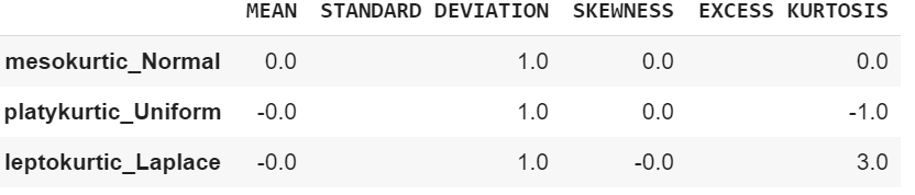
It can be seen above that all the three standardized distributions have roughly the same mean (0) and standard deviation (1) and the skewness of almost 0* i.e. they are symmetrically distributed around their means.
However, when we look at the plot, we see that they are very different distributions and the mean, the standard deviation and the skewness failed to capture this difference in the shape of the distributions. This is where kurtosis comes into the picture.
We can observe in the above figure that the Laplace distribution (green plot) has a leptokurtic distribution and has fatter tails compared to the standard normal distribution (blue plot), which is also reflected in a large and positive excess kurtosis.
On the other hand, the uniform distribution has much shorter/thinner tails compared to a standard normal distribution, which is summarized by a negative excess kurtosis.
Kurtosis-risk/ tail-risk in financial securities
The normality of the distribution of asset returns is a common assumption in many quantitative finance models. This is a convenient assumption, as the normal distribution can be completely summarized by its mean and standard deviation/variance (and has a skewness and excess kurtosis of 0).
Under the assumption of normality, the standard deviation is often used as the only measure of risk. However, the actual distributions of asset returns are not normal and often display positive excess kurtosis.
Thus, assuming normality can severely underestimate the risk of extreme events as distributions with the same mean, same standard deviations and the same skewness can have very different tail profiles (we saw an example of this in the previous section). This risk is also referred to as 'kurtosis risk' or 'fat-tail risk’.
To capture and estimate the tail risk in a better way, risk managers often use a leptokurtic distribution such as the student's t distribution, which is symmetric like the normal distribution but has fatter tails.
In the following figure we generate and plot sample returns from both the standard normal and t distributions and compare them with the actual standardized returns of Indian Tobacco Company (ITC) for the past five years:

We can see in the above figure that the t distribution is better able to model the returns of the stock compared to normal distribution and at the same time captures the kurtosis/tail risk.
Thus, it is advantageous to use a leptokurtic distribution like the student's t distribution while calculating risk metrics such as the Value-at-risk (VaR) or the expected shortfall.
A common error in interpretation of kurtosis
One of the common misconceptions associated with kurtosis is that it is a measure of 'peakedness', as it is easy for us to think that fatter tails automatically implies higher peaks.
However, this is not always true. Take for example two t distributions, one with 3 degrees of freedom and the other with 10 degrees of freedom, that we plot using the following commands:

We can see from above that although the t_3 distribution has a smaller peak, it has much higher excess kurtosis compared to the t_10 distribution.
Analysing the tail risk in S&P 500 and Bitcoin
A general misconception is that highly volatile securities have a higher tail risk and hence a higher excess kurtosis value. However, this is not always true.
Take, for example, the return series for SPDR S&P 500 ETF and the bitcoin for the past five years, which we fetch in Python using the following commands:
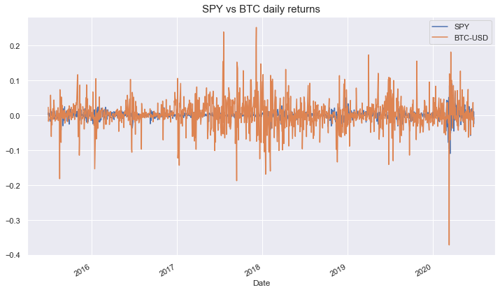
We can clearly see that bitcoin is almost four times more volatile compared to the S&P 500.
Now let us check out the distributions of the two series using the following commands:
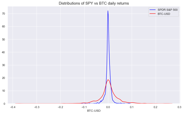
In the above figure, we can see that the two distributions are fairly symmetric around zero with the bitcoin (BTC-USD) returns having a much wider spread (heavier tails), with the extreme values well in excess of 20 percent.
Such magnitudes of extreme values lead to an impression that the bitcoin presents a much higher tail risk compared to the S&P 500. This would naturally imply that the kurtosis value for BTC should well exceed that of S&P 500.
Also, this is in line with the general perception that bitcoin being a cryptocurrency is prone to wild moves giving rise to a higher frequency of observing a tail event compared to equities.
Thus, it is natural that one might think that the distribution of bitcoin will have a higher kurtosis value compared to the S&P 500 equity index. However, when we calculate the excess kurtosis values, we might be in for a surprise:
We see that the kurtosis values above, the SPDR S&P 500 returns have an excess kurtosis which is almost double that of the bitcoin. The reason for this is that the value of kurtosis depends on the departures in the shape of a distribution from the normal distribution.
In order to get more clarity, we should compare the kurtosis of distributions with equal variance, so that we can observe this fact visually. In order to do this, we will first standardise both the distributions such that each one of them has a mean of zero and a variance of one.
Also, we add a third distribution, which is the random sample from a standard normal distribution:
Now, we plot the standardized returns of BTC and S&P 500 along with the random sample from a standard normal distribution:

We can see in the above that the standardized S&P 500 returns (blue) show much more extreme deviations from the standard normal (green). This becomes more evident when we capture these in the density plots using the following commands:
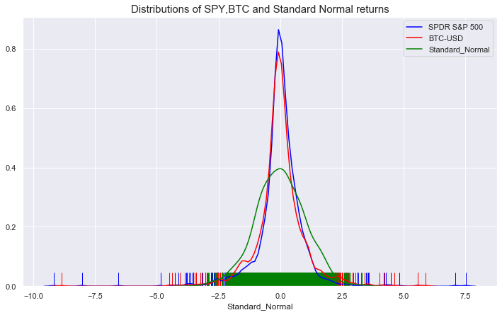
The above figure makes it clear why the standardised SPDR S&P 500 (SPY) returns distribution has a higher kurtosis value compared to the distribution of bitcoin, contrary to the perception.
The reason is the SPY's wider spread (heavier tails) relative to the standard normal distribution i.e. the departure of standardized S&P 500 returns distribution from the standard normal distribution is much more than that of standardized bitcoin (BTC) returns.
Thus, it is important to remember that kurtosis is always calculated relative to the normal distribution and it should be interpreted as such.
Conclusion
In this blog, we have seen how kurtosis/excess kurtosis captures the 'shape' aspect of distribution, which can be easily missed by the mean, variance and skewness. Furthermore, we discussed some common errors and misconceptions in the interpretation of kurtosis.
Kurtosis is a very useful metric to quantify the tail-risk in finance. Ignoring tail-risk can potentially lead to the overestimation of alphas, and hence tail-risk/kurtosis-risk evaluation should be a part of the overall performance evaluation for financial securities.
Similarly, there are other metrics like Kurtosis that if combined with Algorithmic trading can add value to your trading practises. However, if you wish to learn the what, how, why of algorithmic trading, our course on Getting Started with Algorithmic Trading is perfect for you! It not only builds a foundation in Algorithmic Trading but also empowers you with the knowledge of different algorithmic trading strategies and regulations for setting up an algorithmic trading business. Be sure to check it out!
Disclaimer: All investments and trading in the stock market involve risk. Any decisions to place trades in the financial markets, including trading in stock or options or other financial instruments is a personal decision that should only be made after thorough research, including a personal risk and financial assessment and the engagement of professional assistance to the extent you believe necessary. The trading strategies or related information mentioned in this article is for informational purposes only.
File in the zip archive: Complete blog with codes in a Python notebook format
