In this article, we’ll look at data manipulation and visualization techniques in Julia. However, I’ll not get into the details of each parameter of every function, as the objective of this series is to use Julia as a tool to achieve our goal, i.e. building and backtesting trading strategies. So, we’ll stay focused on that.
You can refer to the detailed documentation of a function if you need it to solve any particular challenge you face while programming.
This article is divided into the following sections:
In my previous posts in this Julia programming series, I introduced the language and started with the basic syntax of Julia programming. You can check that out as well.
Data manipulation
You need to understand the data structures dealing with large heterogeneous data sets whenever you work with any programming language. In the Julia world, they are called dataframes.
Julia’s DataFrames.jl package provides a way to structure and manipulate data.
It can be installed using the “Pkg” module.
Creating new dataframes
Here’s an example of creating a new dataframe.
Output:
| Name | Team | Work_experience |
|---|---|---|
| String | String | Int64 |
| Vivek | EPAT | 15 |
| Viraj | Marketing | 8 |
| Rohan | Sales | 7 |
| Ishan | Quantra | 10 |
| a | b |
|---|---|
| Float64 | Float64 |
| 0.845011 | 0.720306 |
| 0.647665 | 0.0409036 |
| 0.427267 | 0.221369 |
| 0.413642 | 0.374832 |
| 0.477994 | 0.118461 |
| 0.0849006 | 0.157679 |
| 0.0477405 | 0.845332 |
| 0.518909 | 0.159305 |
| 0.93499 | 0.259579 |
| 0.60034 | 0.115911 |
Column names can be accessed using the names() function.
Output:

3-element Vector{String}:
"Name"
"Team"
"Work_experience"

3-element Vector{Symbol}:
:Name
:Team
:Work_experience
Renaming columns can be done using the rename() function.
| name | team | work experience |
|---|---|---|
| String | String | Int64 |
| Vivek | EPAT | 15 |
| Viraj | Marketing | 8 |
| Rohan | Sales | 7 |
| Ishan | Quantra | 10 |
Indexing and summarising data
Indexing dataframes to use particular rows or columns for manipulation is a fundamental operation, and summarising data helps us understand it better. In Julia, summary stats of any dataset can be printed using the describe() function.
| variable | mean | min | median | max | nmissing | eltype |
|---|---|---|---|---|---|---|
| Symbol | Float64 | Float64 | Float64 | Float64 | Int64 | DataType |
| a | 0.499846 | 0.0477405 | 0.498452 | 0.93499 | 0 | Float64 |
| b | 0.301368 | 0.0409036 | 0.190337 | 0.845332 | 0 | Float64 |
Another way to find the number of rows and columns in a dataframe is using ncol() and nrow() functions.
Output:
2
10
Let’s look at multiple methods of accessing rows and columns of a dataframe.
Output:
4-element Vector{String}:
"Vivek"
"Viraj"
"Rohan"
"Ishan"

4-element Vector{String}:
"EPAT"
"Marketing"
"Sales"
"Quantra"

3-element Vector{String}:
"EPAT"
"Marketing"
"Sales"
| name | team | work experience |
|---|---|---|
| String | String | Int64 |
| Vivek | EPAT | 15 |
| name | team |
|---|---|
| String | String |
| Vivek | EPAT |
| Viraj | Marketing |
| Rohan | Sales |
| Ishan | Quantra |
Basic mathematical operations
As discussed in my previous post, basic arithmetic operations can be performed on individual columns.
10-element Vector{Float64}:

-0.5474996670806442
 0.5174063588946236
-0.564150142575268
 0.12873854328766576
 0.2741519215981265
 0.20241852864291987
 0.09324017568958975
-0.41716724316286524
 0.2693306887583933
-0.5967498723478988
You’ll have to use the “.” operator for element-wise division.
10-element Vector{Float64}:

0.06754620232737023
3.013387340201863
0.4169119702423886
1.2293455286486041
1.4462537614868343
8.482279426917298
1.1103752688515762
0.21238611891693882
3.1244976300403002
0.38733760512833965
Basic operations
Rearranging columns
r” is a regex search string. Here, any column with a string “work” will be selected and moved to the first place. You can write the full column name as well.
| work experience | name | team |
|---|---|---|
| Int64 | String | String |
| 15 | Vivek | EPAT |
| 8 | Viraj | Marketing |
| 7 | Rohan | Sales |
| 10 | Ishan | Quantra |
Adding a new column in a dataframe
Here we add another column, “c”, to the dataframe df_2.
Dataframe-to-matrix conversion
10×3 Matrix{Float64}:

0.0396604  0.58716    0.741712
0.774389   0.256983   0.429361
0.403371   0.967521   0.989583
0.690069   0.56133    0.50599
0.888493   0.614341   0.152574
0.229472   0.0270531  0.932589
0.937996   0.844756   0.0745573
0.112492   0.52966    0.712178
0.396105   0.126774   0.397762
0.377277   0.974027   0.685073
Grouping data
Let’s look at ways to group data, which comes in handy while summarising data.
In-built datasets in Julia
The package RDatasets.jl in Julia helps you import all the in-build packages in R that can be used for testing purposes.
Here’s how you can find out the list of available datasets. It has 763 datasets.
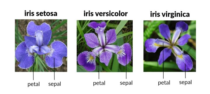
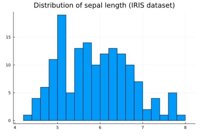
We’ll work with one of the in-built datasets (“iris”) in this section. “iris” provides the data for multiple measurements of 3 plant species and 4 features for each of them. More details about this dataset can be found here.
The following snapshot shows the variables in the iris dataset.
Here’s the summary of this dataset.
| variable | mean | min | median | max | nmissing | eltype |
|---|---|---|---|---|---|---|
| Symbol | Union… | Any | Union… | Any | Int64 | DataType |
| SepalLength | 5.84333 | 4.3 | 5.8 | 7.9 | 0 | Float64 |
| SepalWidth | 3.05733 | 2.0 | 3.0 | 4.4 | 0 | Float64 |
| PetalLength | 3.758 | 1.0 | 4.35 | 6.9 | 0 | Float64 |
| PetalWidth | 1.19933 | 0.1 | 1.3 | 2.5 | 0 | Float64 |
| Species | setosa | virginica | 0 | CategoricalValue{String, UInt8} |
Let’s look at some of the questions you might want to answer using the iris dataset.
We can perform arithmetic operations by grouping data based on various columns. Here’s how we can get the answer to the following question -
What’s the mean value of the sepal length of each species?
| Species | mm |
|---|---|
| Category | Float64 |
| setosa | 5.006 |
| versicolor | 5.936 |
| virginica | 6.588 |
Another package that helps make the operations more intuitive is Pipe.jl. It lets you write operations as they are performed instead of the backward approach.
| Species | mm | ||||||
|---|---|---|---|---|---|---|---|
| Category | Float64 | ||||||
| setosa | 5.006 | ||||||
| versicolor | 5.936 | ||||||
| virginica | 6.588 |
| Species | nrow |
|---|---|
| Category | Float64 |
| setosa | 50 |
| versicolor | 50 |
| virginica | 50 |
Dealing with missing data
Julia has a “missing” object that is used for unavailable data. You can use skipmissing() function to perform operations ignoring the missing values.
Output:
| a | b |
|---|---|
| Int64? | String? |
| 1 | Apple |
| missing | Orange |
| 3 | missing |
| 7 | Grapes |
You can use dropmissing() function to remove the missing values.
| a | b |
|---|---|
| Int64 | String |
| 1 | Apple |
| 7 | Grapes |
More details for dealing with missing values can be found here.
Importing and exporting data as CSV and Excel files
Reading data is the first step in analysing any kind of data. Most of the information we come across is either in CSV or excel format, so we’ll focus on these two. We will work with CSV.jl and XLSX.jl for dealing with CSV and Excel files.
Reading and writing CSV files
We’ll read a CSV file (infy.csv), as a dataframe, containing historical stock price data for Infosys downloaded from Yahoo finance for the period 21-Dec-2020 to 22-Dec-2021.
Here’s a summary for this data.
| variable | mean | min | median | max | nmissing | eltype |
|---|---|---|---|---|---|---|
| Symbol | Union… | Any | Union… | Any | Int64 | DataType |
| Date | 2020-12-22 | 2021-12-21 | 0 | Date | ||
| Open | 20.5674 | 16.39 | 20.63 | 24.05 | 0 | Float64 |
| High | 20.7164 | 16.69 | 20.775 | 24.5 | 0 | Float64 |
| Low | 20.4097 | 16.36 | 20.51 | 23.94 | 0 | Float64 |
| Close | 20.5685 | 16.58 | 20.725 | 24.22 | 0 | Float64 |
| Adj Close | 20.3422 | 16.2664 | 20.5451 | 24.22 | 0 | Float64 |
| Volume | 7.09982e6 | 1320600 | 6.43815e6 | 22911800 | 0 | Int64 |
Here, we calculate the range -
| Date | Open | High | Low | Close | Adj Close | Volume | range |
|---|---|---|---|---|---|---|---|
| Date | Float64 | Float64 | Float64 | Float64 | Float64 | Int64 | Float64 |
| 2020-12-22 | 16.39 | 16.74 | 16.36 | 16.58 | 16.2664 | 6714400 | 0.379999 |
| 2020-12-23 | 16.9 | 16.93 | 16.57 | 16.59 | 16.2762 | 5913500 | 0.36 |
| 2020-12-24 | 16.68 | 16.69 | 16.52 | 16.6 | 16.286 | 1320600 | 0.170001 |
| 2020-12-28 | 16.73 | 16.84 | 16.72 | 16.77 | 16.4528 | 4239300 | 0.120001 |
| 2020-12-29 | 16.9 | 16.9 | 16.67 | 16.76 | 16.443 | 8473700 | 0.23 |
| 2020-12-30 | 16.87 | 17.0 | 16.83 | 16.93 | 16.6098 | 3877200 | 0.17 |
| 2020-12-31 | 17.01 | 17.03 | 16.89 | 16.95 | 16.6294 | 3693700 | 0.140002 |
| 2021-01-04 | 17.39 | 17.43 | 17.06 | 17.25 | 16.9237 | 12597600 | 0.370001 |
| 2021-01-05 | 17.32 | 17.67 | 17.32 | 17.65 | 17.3162 | 8109900 | 0.35 |
| 2021-01-06 | 17.4 | 17.79 | 17.34 | 17.73 | 17.3946 | 9136300 | 0.450001 |
| 2021-01-07 | 17.36 | 17.55 | 17.26 | 17.55 | 17.2181 | 10272000 | 0.289999 |
| 2021-01-08 | 18.07 | 18.61 | 18.02 | 18.59 | 18.2384 | 17802400 | 0.590001 |
| 2021-01-11 | 18.68 | 18.86 | 18.55 | 18.76 | 18.4052 | 12220600 | 0.310002 |
| 2021-01-12 | 18.92 | 18.94 | 18.54 | 18.6 | 18.2482 | 10629100 | 0.4 |
| 2021-01-13 | 19.03 | 19.07 | 18.4 | 18.43 | 18.0814 | 18409900 | 0.67 |
| 2021-01-14 | 18.57 | 18.65 | 18.14 | 18.22 | 17.8754 | 13286100 | 0.510001 |
| 2021-01-15 | 18.19 | 18.38 | 18.11 | 18.17 | 17.8263 | 7443000 | 0.269998 |
| 2021-01-19 | 18.08 | 18.18 | 17.95 | 18.12 | 17.7773 | 7179600 | 0.229999 |
| 2021-01-20 | 18.37 | 18.47 | 18.29 | 18.4 | 18.052 | 5408500 | 0.179998 |
| 2021-01-21 | 18.39 | 18.4 | 18.15 | 18.2 | 17.8558 | 7963400 | 0.25 |
| 2021-01-22 | 18.23 | 18.27 | 18.06 | 18.18 | 17.8361 | 5663500 | 0.210001 |
| 2021-01-25 | 18.15 | 18.22 | 17.84 | 17.92 | 17.5811 | 6012600 | 0.379999 |
| 2021-01-26 | 17.92 | 17.92 | 17.75 | 17.85 | 17.5124 | 5472600 | 0.17 |
| 2021-01-27 | 17.65 | 17.89 | 17.44 | 17.47 | 17.1396 | 11388300 | 0.449998 |
| 2021-01-28 | 17.46 | 17.75 | 17.41 | 17.64 | 17.3064 | 7877600 | 0.34 |
| 2021-01-29 | 17.16 | 17.23 | 16.88 | 16.88 | 16.5607 | 9671400 | 0.350001 |
| 2021-02-01 | 17.19 | 17.42 | 17.05 | 17.38 | 17.0513 | 5829200 | 0.370001 |
| 2021-02-02 | 17.45 | 17.51 | 17.34 | 17.44 | 17.1101 | 4119800 | 0.17 |
| 2021-02-03 | 17.6 | 17.75 | 17.49 | 17.65 | 17.3162 | 4677800 | 0.26 |
| 2021-02-04 | 17.54 | 17.64 | 17.36 | 17.59 | 17.2573 | 4439600 | 0.279998 |
| ⋮ | ⋮ | ⋮ | ⋮ | ⋮ | ⋮ | ⋮ | ⋮ |
This updated dataframe can be saved using CSV.write() function.
Reading and writing excel files
We’ll use the XLSX.jl package in Julia to read and write excel files.
Here’s how it can be done -
| Date | Open | High | Low | Close | Adj Close | Volume |
|---|---|---|---|---|---|---|
| Any | Any | Any | Any | Any | Any | Any |
| 2020-12-22 | 16.39 | 16.74 | 16.36 | 16.58 | 16.2664 | 6714400 |
| 2020-12-23 | 16.9 | 16.93 | 16.57 | 16.59 | 16.2762 | 5913500 |
| 2020-12-24 | 16.68 | 16.69 | 16.52 | 16.6 | 16.286 | 1320600 |
| 2020-12-28 | 16.73 | 16.84 | 16.72 | 16.77 | 16.4528 | 4239300 |
| 2020-12-29 | 16.9 | 16.9 | 16.67 | 16.76 | 16.443 | 8473700 |
| 2020-12-30 | 16.87 | 17.0 | 16.83 | 16.93 | 16.6098 | 3877200 |
| 2020-12-31 | 17.01 | 17.03 | 16.89 | 16.95 | 16.6294 | 3693700 |
| 2021-01-04 | 17.39 | 17.43 | 17.06 | 17.25 | 16.9237 | 12597600 |
| 2021-01-05 | 17.32 | 17.67 | 17.32 | 17.65 | 17.3162 | 8109900 |
| 2021-01-06 | 17.4 | 17.79 | 17.34 | 17.73 | 17.3946 | 9136300 |
| 2021-01-07 | 17.36 | 17.55 | 17.26 | 17.55 | 17.2181 | 10272000 |
| 2021-01-08 | 18.07 | 18.61 | 18.02 | 18.59 | 18.2384 | 17802400 |
| 2021-01-11 | 18.68 | 18.86 | 18.55 | 18.76 | 18.4052 | 12220600 |
| 2021-01-12 | 18.92 | 18.94 | 18.54 | 18.6 | 18.2482 | 10629100 |
| 2021-01-13 | 19.03 | 19.07 | 18.4 | 18.43 | 18.0814 | 18409900 |
| 2021-01-14 | 18.57 | 18.65 | 18.14 | 18.22 | 17.8754 | 13286100 |
| 2021-01-15 | 18.19 | 18.38 | 18.11 | 18.17 | 17.8263 | 7443000 |
| 2021-01-19 | 18.08 | 18.18 | 17.95 | 18.12 | 17.7773 | 7179600 |
| 2021-01-20 | 18.37 | 18.47 | 18.29 | 18.4 | 18.052 | 5408500 |
| 2021-01-21 | 18.39 | 18.4 | 18.15 | 18.2 | 17.8558 | 7963400 |
| 2021-01-22 | 18.23 | 18.27 | 18.06 | 18.18 | 17.8361 | 5663500 |
| 2021-01-25 | 18.15 | 18.22 | 17.84 | 17.92 | 17.5811 | 6012600 |
| 2021-01-26 | 17.92 | 17.92 | 17.75 | 17.85 | 17.5124 | 5472600 |
| 2021-01-27 | 17.65 | 17.89 | 17.44 | 17.47 | 17.1396 | 11388300 |
| 2021-01-28 | 17.46 | 17.75 | 17.41 | 17.64 | 17.3064 | 7877600 |
| 2021-01-29 | 17.16 | 17.23 | 16.88 | 16.88 | 16.5607 | 9671400 |
| 2021-02-01 | 17.19 | 17.42 | 17.05 | 17.38 | 17.0513 | 5829200 |
| 2021-02-02 | 17.45 | 17.51 | 17.34 | 17.44 | 17.1101 | 4119800 |
| 2021-02-03 | 17.6 | 17.75 | 17.49 | 17.65 | 17.3162 | 4677800 |
| 2021-02-04 | 17.54 | 17.64 | 17.36 | 17.59 | 17.2573 | 4439600 |
| ⋮ | ⋮ | ⋮ | ⋮ | ⋮ | ⋮ | ⋮ |
We can write an excel file using the writetable() function.
Julia has in-built read() and write() open() close() functions to work with text files. More details can be found here.
Data can be written in .jld format as well. .jld is Julia’s data format built using the JLD.jl package.
Details for the following packages can be found here -
Data visualization
Data visualization is crucial for understanding and analysing data. We’ll now look at some of the plots using Plots.jl. Plots.jl is one of the commonly used plotting libraries in Julia.
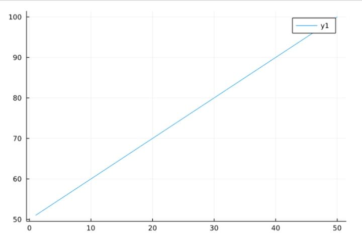
Line plot
Here’s a simple line plot.
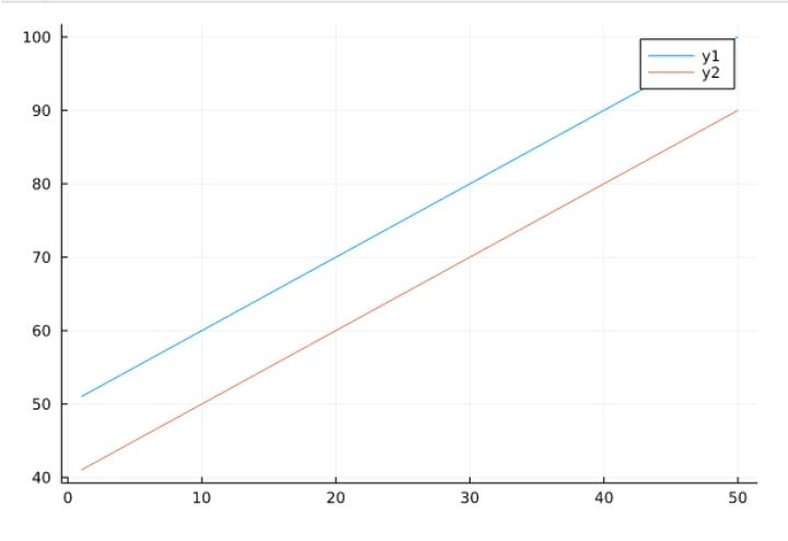
Attributes of a plot
The following attributes can be added to the plot. These attributes can be used for all the plots discussed in this article.
- xlabel - For x-axis label
- ylabel - For y-axis label
- title - Title of the plot
- ylims - Range of y-axis
- xlims - Range of the x-axis
- label - Label names in the legend
- linewidth/lw - For adjusting the width of the line
- color - For adding specific colours to the lines
- legend - Require legend or not and position of the legend. It can take: “topleft”, “topright”, “bottomleft”, “bottomright”, “right”, “bottom”, “top”, “right”, true, false
- layout - For adding multiple plots in the same image.
- size - Size of the plot
This list is not exhaustive; many attributes can be used. However, as I have mentioned earlier, we’ll stay focused on the question: How do we use Julia to achieve our goal?
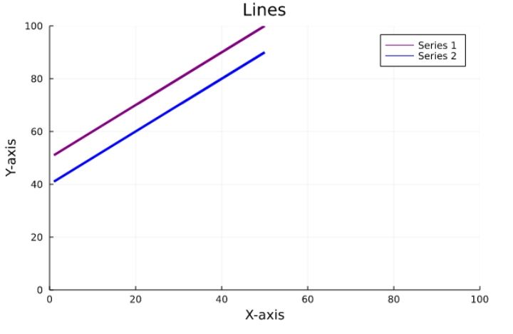
The attributes presented above are most commonly used and should suffice for creating plots.
Here’s an example that combines all the features mentioned above.
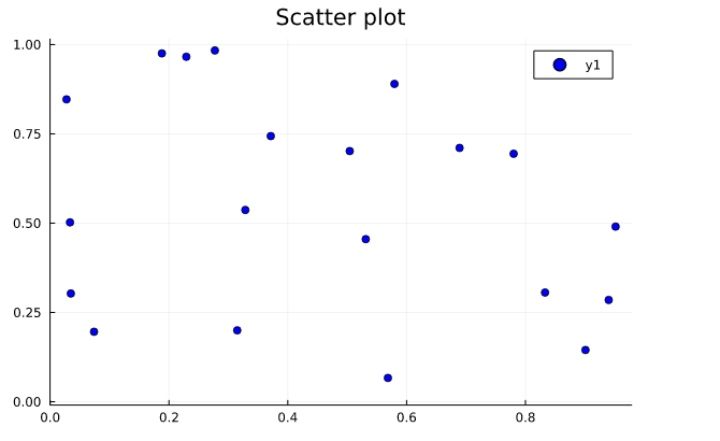
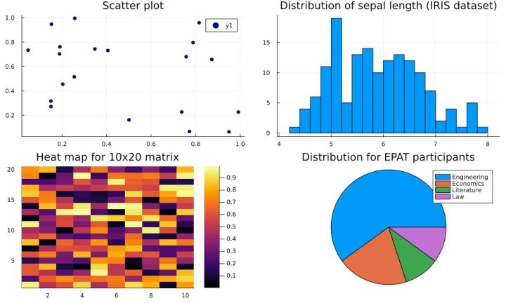
Scatter plot
Scatter plots can be generated using multiple methods. Here are a few examples -
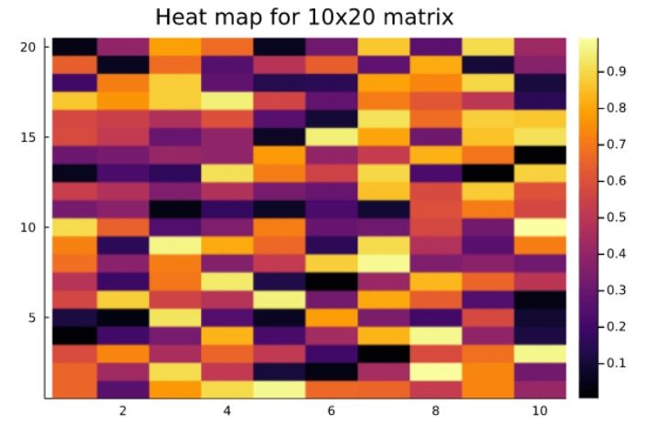
Heatmap
Histogram
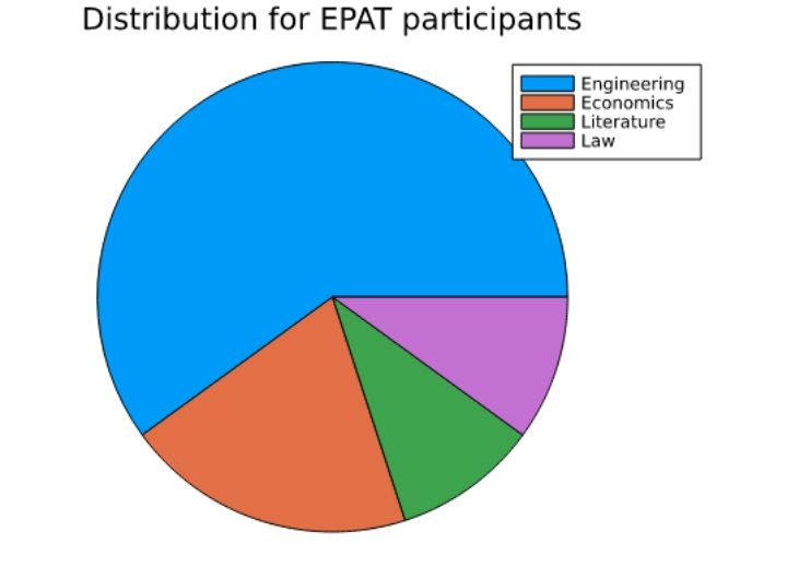
Pie chart
Here’s a sample layout with different plots.
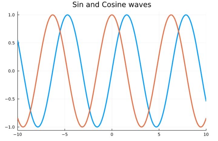
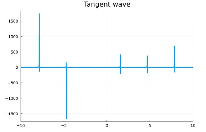
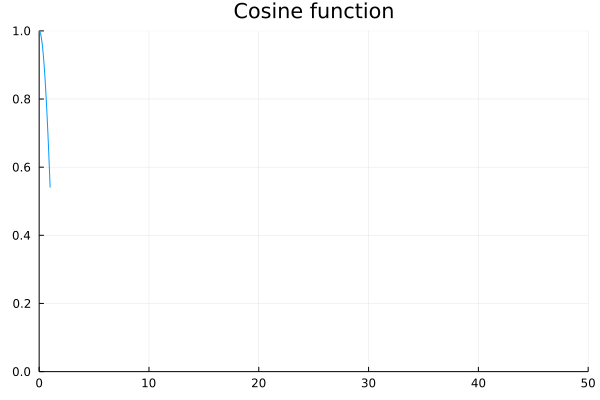
Plotting mathematical functions
Here are some plots of mathematical functions.
Saving plots
The plot generated can be saved in various formats using the savefig() function.
Animated plots
We can also use the plots and covert and save them as gifs or videos.

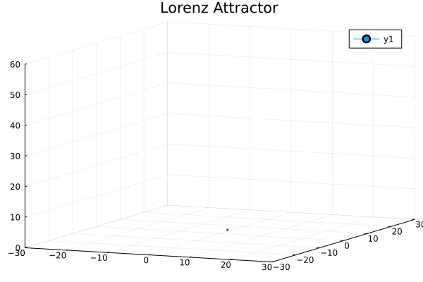
Lorenz attractor
The following is the code of the Lorenz attractor as seen in the Julia documentation:
More details about animated plots can be found here.
Various packages for plotting in Julia
Plots.jl is the basic plotting library in Julia. There are other packages for visualization such as -
- GadFly.jl
- GoogleCharts.jl
- Makie.jl
- PyPlot.jl
- PGFPlotsX.jl
- UnicodePlots.jl and
- VegaLite.jl
Conclusion
This article covers the foundations of data manipulation and visualization using Julia.
In the following article, we’ll look at methods to get timeseries data for stock prices and analyse it using the tools presented in this article. Until then, take this article as a building block and explore the aspects you found interesting in detail!
However, if you are looking to pursue and venture into algorithmic trading then our comprehensive algo trading course taught by industry experts, trading practitioners and stalwarts like Dr. E. P. Chan, Dr. Euan Sinclair to name a few - is just the thing for you. Enroll now!
Author: Anshul Tayal
Disclaimer: All data and information provided in this article are for informational purposes only. QuantInsti® makes no representations as to accuracy, completeness, currentness, suitability, or validity of any information in this article and will not be liable for any errors, omissions, or delays in this information or any losses, injuries, or damages arising from its display or use. All information is provided on an as-is basis.