
By Vibhu Singh, Varun Divakar and Ashish Garg
This blog covers the Hurst exponent, a crucial concept in time series analysis, which helps in identifying whether a time series is mean-reverting, random, or trending. Before diving into this topic, it is essential to build a strong foundation in time series concepts.
Pre requisites
Start with Introduction to Time Series, which explains the fundamentals of time series, its importance in financial markets, and various forecasting techniques.
By familiarizing yourself with these foundational concepts, you'll be better equipped to interpret the significance of the Hurst exponent and apply it effectively in trading and investment strategies.
Hurst Exponent Definition
The Hurst exponent is used as a measure of long-term memory of time series. It relates to the autocorrelations (You can read more about Autocorrelation and Autocovariance.) of the time series and the rate at which these decrease as the lag between pairs of values increases.
Hurst Value
Hurst Value is more than 0.5
If the Hurst value is more than 0.5 then it would indicate a persistent time series (roughly translates to a trending market).
Hurst Value is less than 0.5
If the Hurst Value is less than 0.5 then it can be considered as an anti-persistent time series (roughly translates to sideways market).
Hurst Value is 0.5
If the Hurst value is 0.5 then it would indicate a random walk or a market where prediction of future based on past data is not possible.
How To Calculate The Hurst Exponent
To calculate the Exponent, we need to divide the data into different chunks. For example, if you have the return data of BTC/USD for the past 8 days’ data, then you divide it into halves as follows.
Following the example of 8 observations for illustrative purposes only1:
| Data | Chunk 1 |
| 0.04 | |
| 0.02 | |
| 0.05 | |
| 0.08 | |
| 0.02 | |
| -0.17 | |
| 0.05 | |
| 0 |
1Length of the subseries in practical applications is usually much longer and affects the mean and standard deviation of the R/S statistic.
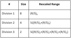
Then, we divide the data into 3 different chunks as follows:
- Division 1 - one chunk of 8 observations
- Division 2 - two chunks of 4 observations each
- Division 3 - four chunks of 2 observations each
| Data | Chunk 1 |
| 0.04 | |
| 0.02 | |
| 0.05 | |
| 0.08 | |
| 0.02 | |
| -0.17 | |
| 0.05 | |
| 0 |
| Data | Chunk 2 | Chunk 3 |
| 0.04 | 0.02 | |
| 0.02 | -0.17 | |
| 0.05 | 0.05 | |
| 0.08 | 0 |
| Data | Chunk 4 | Chunk 5 | Chunk 6 | Chunk 7 |
| 0.04 | 0.05 | 0.02 | 0.05 | |
| 0.02 | 0.08 | -0.17 | 0 |
After dividing the data into chunks, we perform the following calculations on each chunk:
Step 1
First we calculate the mean of the chunk, with say n observations,
M = (1/n) [ h(1)+h(2)+...+h(n) ]
| Data | Chunk 1 |
| 0.04 | |
| 0.02 | |
| 0.05 | |
| 0.08 | |
| 0.02 | |
| -0.17 | |
| 0.05 | |
| 0 |
| Data | Chunk 2 | Chunk 3 |
| 0.04 | 0.02 | |
| 0.02 | -0.17 | |
| 0.05 | 0.05 | |
| 0.08 | 0 |
| Data | Chunk 4 | Chunk 5 | Chunk 6 | Chunk 7 |
| 0.04 | 0.05 | 0.02 | 0.05 | |
| 0.02 | 0.08 | -0.17 | 0 |
Step 2
Then we calculate the standard deviation (S) of the n observations
s(n) = STD( h(1),h(2),...,h(n))
| Mean | 0.01 |
| Std | 0.08 |
| Mean | 0.05 | -0.03 |
| Std | 0.03 | 0.10 |
| Mean | 0.03 | 0.07 | -0.08 | 0.03 |
| Std | 0.01 | 0.02 | 0.13 | 0.04 |
Step 3
Then we create a mean centered series by subtracting the mean from the observations,
x(1) = h(1) - M x(2) = h(2) - M ... x(n) = h(n) - M
| Mean-centred series | 0.03 |
| 0.01 | |
| 0.04 | |
| 0.07 | |
| 0.01 | |
| -0.18 | |
| 0.04 | |
| -0.01 |
| Mean-centred series | -0.01 | 0.05 |
| -0.03 | -0.15 | |
| 0.00 | 0.08 | |
| 0.03 | 0.03 |
| Mean-centred series | 0.01 | -0.02 | 0.10 | 0.03 |
| -0.01 | 0.02 | -0.10 | -0.03 |
Step 4
Then we calculate the cumulative sum of the mean-centred deviations. This cumulative series is obtained by adding the mean-centred values sequentially.
Y(1) = x(1) Y(2) = x(1) + x(2) ... Y(n) = x(1) + x(2) + ...+ x(n)
| Cumulative sum of Mean-centred series | 0.03 |
| 0.04 | |
| 0.08 | |
| 0.15 | |
| 0.15 | |
| -0.03 | |
| 0.01 | |
| 0.00 |
| Cumulative sum of Mean-centred series | -0.01 | 0.05 |
| -0.04 | -0.10 | |
| -0.03 | -0.03 | |
| 0.00 | 0.00 |
| Cumulative sum of Mean-centred series | 0.01 | -0.02 | 0.01 | 0.03 |
| 0.00 | 0.00 | 0.00 | 0.00 |
Step 5
Next, we calculate the Range (R), which is the difference between the maximum and minimum values of the cumulative sum series calculated in Step 4:
| Range | 0.18 |
| Range | 0.04 | 0.15 |
| Range | 0.01 | 0.02 | 0.10 | 0.03 |
Note: Here, “cumulative sum” refers to the running sum of the mean-centred deviations.
Step 6
And finally, we compute the ratio of the range R to the standard deviation S. This also known as the rescaled range.
| Range | 0.18 |
| R/S (Range/ Std) | 2.35 |
| Range | 0.04 | 0.15 |
| R/S (Range/ Std) | 1.40 | 1.47 |
| Range | 0.01 | 0.02 | 0.10 | 0.03 |
| R/S (Range/ Std) | 0.71 | 0.71 | 0.71 | 0.71 |
Step 7
Once we have the rescaled range for all the chunks, we compute the mean of each Division and note it along with the number of samples in each chunk of that Division as shown.
| Range | 0.18 |
| R/S (Range/ Std) | 2.35 |
| Average R/S | 2.35 |
| Range | 0.04 | 0.15 |
| R/S (Range/ Std) | 1.40 | 1.47 |
| Average R/S | 1.43 |
| Range | 0.01 | 0.02 | 0.10 | 0.03 |
| R/S (Range/ Std) | 0.71 | 0.71 | 0.71 | 0.71 |
| Average R/S | 0.71 |
Step 8
Next, we calculate the logarithmic values for the size of each region and for each region’s rescaled range.
| Summary | |||
| Size | R/S | Log of Size | Log of R/S |
| 8 | 2.35 | 2.08 | 0.85 |
| 4 | 1.43 | 1.39 | 0.36 |
| 2 | 0.71 | 0.69 | -0.35 |
Result
The Hurst exponent ‘H’ is nothing but the slope of the plot of each range’s log(R/S) versus each range’s log(size).
Here log(R/S) is the dependent or the y variable and log(size) is the independent or the x variable:
| Hurst Exponent | 0.87 |
Conclusion
This hurst exponent value is indicating that our data is a persistent one, but we have to keep in mind that our data set is too small to draw such a conclusion.
For example, if you want to calculate hurst exponent in python using the ‘hurst’ library, it requires you to give at least 100 data points.
We hope you have learnt how to calculate the Hurst exponent from this blog. In our advanced course on cryptocurrencies, we have demonstrated how hurst exponent along with another technical indicator can yield optimized trading signals.
Next steps
Now that you have learnt about Hurst Exponent and Time series, let's dive deeper into Mean Reversion in time series to understand how and why time‐series data exhibit long‐term memory.
Once you’re comfortable with these, progress to advanced or multivariate methods, including Vector Autoregression (VAR), Johansen Cointegration, and Time-Varying-Parameter VAR.
This comprehensive roadmap equips you with the necessary background to fully appreciate this Blog. You are expected to know how to use these models to forecast time series. You should also have a basic understanding of R or Python for time series analysis.
Strengthen your grasp by looking into Autocorrelation & Autocovariance to see how data points relate over time, then deepen your knowledge with fundamental models such as Autoregression (AR), ARMA, ARIMA and ARFIMA.
If your goal is to discover alpha, you may want to experiment with a variety of techniques, such as technical analysis, trading risk management, pairs trading basics, and Market microstructure. By combining these approaches, you can develop and refine trading strategies that better adapt to market dynamics.
Check out this learning track on Algorithmic Trading in Cryptocurrency and Forex, this covers Hurst exponent strategy. Also, you can check out the new course on Quant Investing for Portfolio Managers, Generalized Hurst Exponent. You will learn the Generalized Hurst Exponent as a tool to analyse market trends, identify momentum, and refine factor timing strategies.
For a structured approach to algo trading and to master advanced statistics for quant strategies consider the best algorithmic trading course, the Executive Programme in Algorithmic Trading (EPAT). This rigorous course covers time series fundamentals (stationarity, ACF, PACF), advanced modelling (ARIMA, ARCH, GARCH), and practical Python‐based strategy building, providing the in‐depth skills needed to excel in today’s financial markets.
Disclaimer: All investments and trading in the stock market involve risk. Any decisions to place trades in the financial markets, including trading in stock or options or other financial instruments is a personal decision that should only be made after thorough research, including a personal risk and financial assessment and the engagement of professional assistance to the extent you believe necessary. The trading strategies or related information mentioned in this article is for informational purposes only.
