In this article, we will study a deep learning framework based on recurrent neural networks to predict daily equity index price movements. Specifically, the focus will be on long short-term memory (LSTM) networks - which are a type of recurrent neural network.
Different types of inputs and network architectures will be studied to determine their effect on predictability. We will see that with a suitable combination of inputs and architecture, a strategy with a Sharpe ratio higher than a simple buy-and-hold approach can be developed.
Differences, limitations and factors that need to be considered compared to a traditional machine learning approach will also be highlighted. After going through the article, the reader should be able to create a basic LSTM-based neural network to predict price movements of any instrument with ease based on publicly available data. Learn more about the applications and role of neural network in trading to enhance your skills.
This article is the final project submitted by the authors as a part of their coursework in the Executive Programme in Algorithmic Trading (EPAT®) at QuantInsti®. Do check our Projects page and have a look at what our students are building.
About the Author

Dr. Krishna Tunga holds a Bachelor’s degree from IIT-Madras, Masters and Doctorate degrees from Georgia Tech - all in Engineering. His areas of interests include Semiconductors, Reliability and risk prediction, Modeling and Simulation, Artificial Intelligence, Machine Learning, Deep Learning, Finance and Financial Derivatives.
Overview
It is reasonable to expect an equity index to move in accordance with the prevalent and anticipated macroeconomic outlook. However, recent work by Nobel laureates Tversky and Kahneman[1] has demonstrated that behavioural biases are pervasive with traders and investors and could lead to persistence in price movement that could last for days, weeks or even months.This makes predicting future prices based on historical price (and volume) changes a possibility.
Numerous technical indicators that fall under the broader category of overlap indicators, momentum indicators, volatility indicators etc. have been used for several decades for predicting price movement.
Recent advances in computational power have made it possible to use traditional supervised machine learning methods such as support vector machines, decision trees, principal component analysis, random forest, ensemble methods etc. to predict future prices by using combinations of several technical indicators along with prices as inputs.
One of the drawbacks with traditional machine learning methods mentioned above is that they all require manually picking indicators, based on a preconceived hypothesis of the picked indicator as having a predictive power, calculating them beforehand and then using them as independent predictors in a machine learning model.
Such a hypothesis might not always be correct, and it is not possible to determine an ideal set of independent predictors to use by trial-and-error since the number of such possible combinations to test for is theoretically infinite.
Recurrent Neural Networks (RNN), which is one of the supervised machine learning methods, can potentially resolve this issue. A very good theoretical overview of RNN’s has been provided by Christopher Olah[2] and will not be dealt with in this article.
Central to the concept of RNN is a cell which possesses a persistent internal state based on historical price changes. The cell is first initialized to a random state and takes input data in the form of the price (or volume or any other data as appropriate) that is fed into the cell sequentially at definite and regular time intervals.
As each input data is fed to the cell, one by one, the state of the cell changes and this changed state is conveyed back to the cell at the next time sequence along with the new input data. The state of the cell therefore constantly changes with time-based on its previous state and new input data.
All historical movements in the input data are therefore in some way ‘comprehended’ by the cell and are represented by its current state. There is hence no need to separately calculate beforehand all technical indicators, based on hypothesis, and feed to the model as predictors though it can be added to the input data if so desired.
Long Short-Term Memory (LSTM) networks are an enhancement to RNNs, developed by Hochreiter & Schmidhuber in 1997. LSTMs can learn longer duration dependencies in addition to short duration dependencies like RNNs. They are able to achieve this by introducing three gates - forget gate, update gate and output gate - that dictate respectively:
a. the fraction of the previous internal state of the cell that should be retained,
b. the fraction of the new input data and previous output data that should be retained and added to the previous internal state and
c. the fraction of the current internal state that should be used to determine the output and transmitted to the next cell along with the current internal state.
These fractions are determined by fitting and calibrating the model with known historical inputs to known output labels or label values. This is, of course, a very simplistic overview of LSTMs. For a more detailed explanation, the reader is advised to read ref[2].
All of this comes with an added computational cost. LSTMs are therefore known to be computationally expensive and running these models on a machine with enough GPU cores would be helpful.
Data and Base Network Description
In the first part of this study, I will first use a base LSTM network, as shown below in Figure 1, to predict the average daily return of the SPY index for the next 3 days using the previous 3 months of price data as input – all based on adjusted closing prices. The entire network was scripted using Keras library and Python 3.7.
The input data used for this work was the daily price return of the SPY index from Jan 2nd 1998 to Dec 19th, 2019 downloaded from Yahoo. The first 90% of the historical data was used for training the network and the last 10% of the data was used for validation.
The return data for the training set was converted to z-scores, by fitting and transforming the set using the StandardScaler().fit_transform() function from sklearn.preprocessing, before using them as inputs into the model.
The return data for the validation set was transformed using the fitted mean and standard deviation as determined from the training set data.
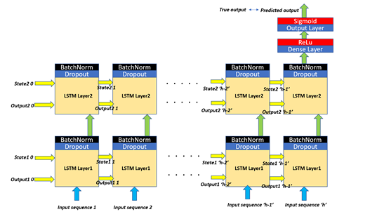
The base structure had two LSTM layers. The cell state and cell output for both the layers were represented using 64 nodes. The initial cell state (State1 0, and State 2 0) and the cell output (Output1 0 and Output2 0) for both the layers were set to the default option provided by Keras.
Layer 1 took as input the fit-transformed historical price return data, described before, for the past 60 days as a sequence.
The output from layer 1 was fed into a dropout layer with 20% dropout to reduce overfitting and over-dependence on only a few nodes within the layer.
The output from the dropout layer was fed to a batch-normalization layer to avoid co-variance shift from affecting the model.
Batch-normalization also has a slight regularization effect which tends to reduce overfitting as well. The output from LSTM layer 1 is fed to LSTM layer 2 followed by another layer of dropout and batch-normalization layer.
The output from the last cell of the second LSTM layer was then fed into a Dense layer with 32 nodes followed by a Rectified Linear (ReLu) activation function which is known to increase the rate of learning.
The output from this Dense layer was then fed to the final output layer with just one node followed by a Sigmoid activation which provides an output value between 0 and 1.
The output from the Sigmoid function was compared to the true output and the model loss was calculated using ‘binary_crossentropy’. The true output was the binarized version of the average daily return for the next 3 days with the output set to 1 if the return was positive and output set to 0 if the return was negative.
Keras automatically performs backpropagation to minimize losses from the training data and determines the weights accordingly. Adam optimizer with the default learning rate of 0.001 and learning rate decay of 1e-6 was used for fitting the model. The model was run for 100 epochs with a batch size of 128.
Base Network Results
LSTM networks arrive at the optimal weights using backpropagation. The entire process is stochastic in nature. This brings about some amount of randomness in the estimated weights and in the predicted output.
Randomness is also introduced by the choice of random weights used to initialize the cell states and the weight matrices. The randomness in output is one of the drawbacks of neural networks and generally decreases when the fitted loss from the model is low (or when the fitted accuracy is high).
For this study, to get rid of randomness and even out the non-deterministic part, the same model was run 10 times. Both the mean and the deviation of the outputs from the 10 runs were used to assess the quality and usefulness of the fitted model.
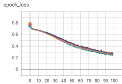
Variation of loss from the model fit as a function of a number of epochs trained for is shown in Figure 2 for both the training set (left plot) and validation set (right plot).
Backpropagation with Adam optimizer has done a good job in reducing the losses of the fitted model with the training set data. However, when the fitted model was used with the validation data for verification, we can see that the losses increase with the number of epochs and are considerably higher than the losses that were seen with the training set.
Since the losses are not minimized, we can also see a considerable variation in losses between the 10 different model runs amounting to a standard deviation of about 10%. All of this indicates that the model has very likely overfitted to the training data and therefore not doing a good job with the validation set.
However, keep in mind that for signal generation, we don’t necessarily need the model to have a low level of loss or high level of accuracy. If the model can generate good signals with more than 50% accuracy, it can still be profitable if the amount of gains from the correct signals is higher than the number of losses from the false ones.
The LSTM model that was used was basically a binary classifier that outputs a value between 0 and 1 which is then discretized to either 0 or 1 for a sell signal (negative) and a buy signal (positive) respectively.
This means we can look at other metrics such as – precision, recall (sensitivity) and f1score – to assess the performance of the model. Precision indicates the fraction of the buy signals predicted by the model that actually were true buy signals. Recall quantifies the effectiveness of the model in predicting the true buy signals.
In other words, it indicates the fraction of the true buy signals that were correctly predicted by the model. F1score is just the harmonic mean between precision and recall and combines both these metrics into one metric. If all three of these metrics are greater than 0.5, the model has the potential to be profitable.
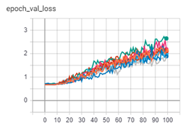
Plots showing the variation of all three of these metrics for both the training set and validation set is given in Figure 3.
All three metrics increase with the number of epochs for the training set data and are more than 0.9 with 100 epochs of training. However, these metrics are significantly lower when tested with the validation data and appears to have reached a plateau at around 50 epochs. The average plateau levels are, however, higher than 0.5 suggesting that the model might still be useful.
Let’s try to improve upon the model prediction by adding more inputs in addition to the SPY price data input we already are using. Given below are the list of inputs we will use for further study:
a. SPY price data only (base case)
b. SPY price and volume data
c. SPY price and volume and historical volatility data
d. SPY and TLT price and volume data
The volume data was converted using the same approach that was used to convert the price data i.e. first converted to percent change values based on daily close-to-close volumes and then fitted and transformed using the StandardScaler() function from sklearn.
The validation data for volume was transformed using the fitted mean and deviation as determined from the training data. The historical volatility was calculated using the standard deviation of past month prices. The historical volatility values were converted to z-scores - using the fit and transform approach described above – before using them as inputs into the model.
US treasuries have historically served as a safe harbour during risk-off situations when investors typically pull money out of the equity market and put them into the bond market. US treasuries have therefore had a negative correlation with the US equity indices at least for the past couple of decades.
The negative correlation is stronger with the longer-term US treasuries. So, as a final case, I have added the price and volume data of the 20+ year long-term treasury ETF – TLT- as additional inputs (case d) to see if we can obtain a better predicting model.
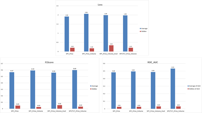
We will look at the validation data set loss and f1score for all four cases above and compare to see if adding additional inputs was helpful. In addition, we will also compare the area under the Receiver Operating Characteristic (ROC) curve – also called AUC - for all four cases above.
ROC curve is commonly used to select an optimal binary classifier system by plotting the benefit vs. cost at various threshold levels. The benefit is equal to the fraction of the positives predicted correctly by the model (true positive rate or sensitivity) and the cost is equal to the fraction of the negatives predicted incorrectly by the model (false positive rate or 1-specificity).
A random binary classifier would give an area under the ROC curve of 0.5. So, for the model to be better than the random classifier, we would want the area under the ROC curve to be greater than 0.5 – the higher the better.
Plots showing the mean and standard deviation (from 10 model runs) of validation data set loss, f1score and ROC-AUC for the four cases above after 100 epochs are given in Figure 4.
Including the volume data in addition to price data led to very marginal increases in f1score and ROC-AUC score at the expense of slightly higher loss. The ROC-AUC is still lower than 0.5 making the model still not very useful. Adding historical volatility data in addition to the volume data did not change the mean ROC-AUC value. Instead, it led to a slight decrease in the f1score making the model slightly worse.
Since historical volatility is derived from price data, it is likely that adding this data did not really provide any additional information beyond what was already provided by the price data. Instead of using historical volatility, if implied volatility was used, the performance could have been better.
This was, however, not studied in this work. Including TLT price and volume data did cause an increase in f1score and ROC-AUC value. The ROC-AUC value was at or higher than 0.5 even after including one standard deviation of possible variation.
The loss was also lower than with the SPY price and volume data alone when used as inputs.
The fitted model for all four of the cases above was used with the validation data set to generate buy/sell signals daily which were then used to either go long or short the SPY index ETF.
The Sharpe ratio of the equity curve generated from trading the buy/sell signals is compared in Figure 5. Daily closing prices were assumed for the trades and the commissions were set to zero. The benchmark used for comparison was the SPY index value (adjusted closing price).
One can see from the plot that using price alone to generate buy/sell signals from the LSTM network leads to degraded performance even after including the deviation from 10 model runs.
Including volume or historical volatility or TLT price/volume data greatly improves the performance. However, statistically, there is not much difference between these three cases. Also, statistically, the Sharpe ratio does not appear to be any better compared to the benchmark.
We will next see if we can improve the model performance by changing the LSTM network architecture.

Network Architecture Variation
There are several ways the LSTM network architecture can be changed including but not limited to, changing the number of LSTM layers, changing the number of nodes to represent the cell state and cell output, changing the number of Dense layers and its nodes, changing the activation function within the LSTM layer and/or within the Dense layer etc.
We will look at two key changes that might affect the network performance considerably:
a) adding an extra LSTM layer beyond the two layers that already exists
b) use three different node sizes within each of the LSTM layers: 32, 64 (current) and 128.
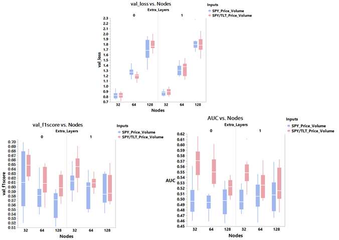
We will compare the same three key metrics – loss, f1score and ROC-AUC – along with the Sharpe ratio for only the last two cases listed in the previous section i.e for SPY price/volume data as inputs and SPY/TLT price/volume data as inputs.
Comparisons of the key metrics, after 50 epochs and with 10 model runs for each scenario, are shown in Figure 6. Adding an extra LSTM layer did not change the validation data loss, f1score or ROC-AUC score appreciably.
Decreasing the number of nodes within each LSTM layer, however, did have a huge impact. With a higher number of nodes, it was very likely that the model was overfitting to the data leading to higher losses.
With fewer nodes, the loss significantly decreased and the f1score significantly increased especially when SPY/TLT price/volume data was used as input. With fewer nodes, the ROC-AUC score improved only when SPY/TLT price/volume was used as the input data. LSTM network with 32 nodes and no extra layer added was, therefore, the best configuration looking at all three metrics.
A comparison of the Sharpe ratio determined from the equity curve that was generated using these different LSTM configurations is shown in Figure 7.
Sharpe ratio improves with fewer nodes when both SPY and TLT data are used as inputs with improvement being the highest when no extra layers are added to the LSTM network.
The configuration with 32 nodes and no extra layer added, again, appears to be the best option.

Historical and Future Period Variation
The analysis that is done so far focused on predicting the average daily return for the next 3 days using the historical price/volume data for the past 3 months.
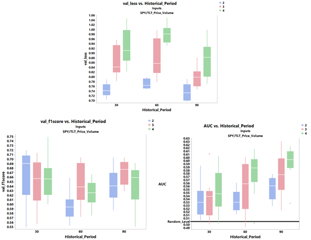
In this section, we will look at varying both these parameters to see if the predictability of the model can be improved further. We will look at three different historical periods – 30, 60 and 90 working days – and three different future periods – 2, 3 and 4 working days.
The number of nodes was kept at 32. The models were run for 50 epochs (since all of the validation metrics had reached a plateau after around 50 epochs) and 10 such simulations were run for each case to determine the mean and standard deviation of all the metrics.
The plots for the key model metrics for the validation data after 50 epochs are shown in Figure 8. The ROC-AUC score improves with longer historical duration and longer future duration with the highest mean value being close to 0.6.
However, this comes at the expense of higher loss as well. The f1score does not appear to follow any predictable trend but all are above 0.6 - which is good.
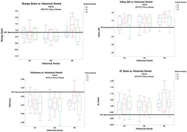
In addition to Sharpe ratio, we will look at three additional return metrics - %maximum drawdown, %winners and PL ratio (ratio or winning returns to losing returns).
Except for the 90-3 (historical periods-future periods) case, the Sharpe ratio for all other cases does not seem to be significantly different from the SPY buy-and-hold benchmark.
However, the %maximum drawdown appears to be much better than the benchmark for all cases with the 90-3 being the best case. The mean %winners are lower than the benchmark (with the 90-3 combination being the best) and the mean PL ratio is higher than the benchmark (with the 90-3 again being the best).
Overall, looking at all four return metrics, 90-3 combination appears to be the best option.
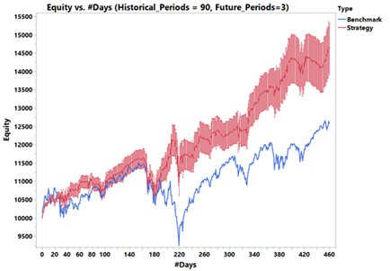
We will now look at the equity curve generated from using the trained 90-3 input-output period combination, two-layered LSTM network with 32 nodes, that took the SPY+TLT price and volume data as inputs and generated buy/sell signals.
These signals were used to trade the SPY index ETF daily using the closing prices, to generate an equity curve - all assuming zero commissions.
The model was run 10 times to account for the stochastic nature of the LSTM network and to obtain an estimate of the standardized error in the generated curve.
A comparison of the generated equity curve with the SPY benchmark is shown in Figure 10. It can be seen from the plot that the strategy does provide superior returns even after accounting for the standardized error in the predicted results.
The validation data set had about 460 trading days and the benchmark returned close to 22% during that time frame. The strategy using LSTM network is predicted to return anywhere from 37.5% to 52.5% during the same time frame.
Summary and Conclusion
In this study, we looked at an enhanced version of the recurrent neural network called the LSTM network to predict SPY equity index prices based on historical price and volume data.
We initially started with a base network and with only SPY price as the input data and got a performance that was worse compared to a simple buy and hold strategy. By adding additional input data related to volume and US long term treasury price/volume data, the predictability was greatly improved.
The network’s performance was further ‘optimized’ and increased by decreasing the number of nodes (to prevent overfitting) and by changing the historical input period and predicted future output period.
So, to answer the question posed in the title of this article: yes, LSTMs can be used to predict future price movement, however, with few caveats as described below.
The advantage of not having to choose and calculate several technical indicators beforehand and feed as input to the model is negated partially at least by having to input several additional parameters that LSTM networks require to define its architecture such as:
- number of LSTM layers,
- number of nodes in each of the layer,
- length of the input sequence,
- number and size of Dense layers,
- type of activation etc
- all of which are called hyperparameters.
Choosing the best architecture, therefore, requires some amount of hyperparametric tuning.
And finding an optimal architecture, as we have done to some extent in this study, might not always guarantee superior signals in the future especially if there is a regime shift that has not been seen before and learnt from the training set.
One way to prevent this from happening is to change the architecture of the network and train it on an ongoing basis using recent data applicable to the current regime and make predictions using the newly trained network.
This will require a lot of computational power!
- LSTM network fits the model using backpropagation, which is a stochastic optimization process requiring random initial guesses for the weights and for the initial cell states.
The optimization is done using some form of stochastic gradient descent process which requires additional hyperparameters that need to be defined for eg: learning rate, learning rate decay, beta1, beta2, regularization parameters, dropout percentage etc.
The fitted model weights could, therefore, be different based on initialized weights and the hyperparameter set that was chosen prior to fitting the model.
Since the model loss as determined using test data is generally always high compared to the loss from the training data, the variability in the estimated weights could also be high between different runs of the same model.
The model should, therefore, be run several times to average out the non-deterministic part of the model and to arrive at a mean estimate of the predicted weights, outputs and return metrics.
This makes providing a buy/sell recommendation time consuming and would require higher computational power especially when used for high-frequency algorithmic trading. - The standard error in the predicted mean results from several model runs is inversely proportional to the square root of the number of runs. So, increasing the number of simulations for the same model should help in arriving at an output that’s more deterministic.
Randomness in the prediction made by the LSTM network can also be partially mitigated by using a random seeder from numpy.random or tensorflow.set_random_seed.
The effect of both was not investigated as part of this study but something that might be useful to study further.
If you want to learn various aspects of Algorithmic trading then check out the Executive Programme in Algorithmic Trading (EPAT). The course covers training modules like Statistics & Econometrics, Financial Computing & Technology, and Algorithmic & Quantitative Trading. EPAT equips you with the required skill sets to build a promising career in algorithmic trading.
Disclaimer: The information in this project is true and complete to the best of our Student’s knowledge. All recommendations are made without guarantee on the part of the student or QuantInsti®. The student and QuantInsti® disclaim any liability in connection with the use of this information. All content provided in this project is for informational purposes only and we do not guarantee that by using the guidance you will derive a certain profit.
References
- Prospect Theory: An Analysis of Decision under Risk, Daniel Kahneman and Amos Tversky, Econometrica, Vol. 47, No 2, pp. 263-292
- https://colah.github.io/posts/2015-08-Understanding-LSTMs/
Files in the download
- Python script - BaseNetwork
- SPY
- TLT