In our previous post on Machine learning we derived rules for a forex strategy using the SVM algorithm in R. In this post we take a step further, and demonstrate how to backtest our findings.
To recap the last post, we used Parabolic SAR and MACD histogram as our indicators for machine learning. Parabolic SAR indicator trails price as the trend extends over time. SAR is below prices when prices are rising and above prices when prices are falling. SAR stops and reverses when the price trend reverses and breaks above or below it.
The MACD oscillator comprises of the MACD line, Signal line and the MACD histogram. The MACD Line is the 12-day Exponential Moving Average (EMA) less the 26-day EMA. MACD Signal line is a 9-day EMA of the MACD line. The MACD Histogram represents the difference between MACD line and the MACD Signal line. The histogram is positive when the MACD Line is above its Signal line and negative when the MACD Line is below its Signal line.
The EUR/USD price series chart below shows Parabolic SAR plotted in blue, and the MACD line, MACD signal line, and the MACD histogram below the EURUSD price series.

Our intention is to take positions around the MACD line crossovers and Parabolic SAR reversal points. When the Parabolic SAR gives buy signal and MACD lines crosses upwards, we buy. When Parabolic SAR gives sell signal and MACD lines crosses downwards, we sell.

After selecting the indicators we ran the SVM algorithm on EUR/USD data, which gave us the plot as shown above. Looking at the SVM predictions, we now frame the rules, and backtest them to see the performance of our strategy.
Short rule = (Price – SAR) < 0.0010 & MACD histogram < 0.0010 Long rule = (Price – SAR) > -0.0050 & MACD histogram > -0.0010
We have used Michael Kapler's Systematic Investor Toolbox to backtest our model in R. We start by loading the toolbox and the necessary libraries.

Next we create a new environment and load the historical EUR/USD data using the getSymbols function.

We will check the performance of our rule-based model against a simple ‘buy and hold’ model. To do that, we first create a ‘buy and hold’ model.

Our next step is to compute the indicators for our rule-based model.

We run two models here, ‘long short’ model, and another ‘long short’ model using stop loss and take profit. First we create a long short model without stop loss and take profit.

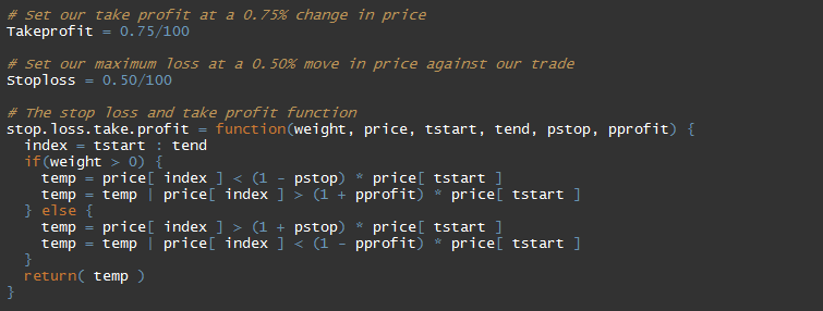
Next we set the takeprofit and stop loss levels, and create a long short model using these levels. We call this model as ‘stop.loss.take.profit’ model.

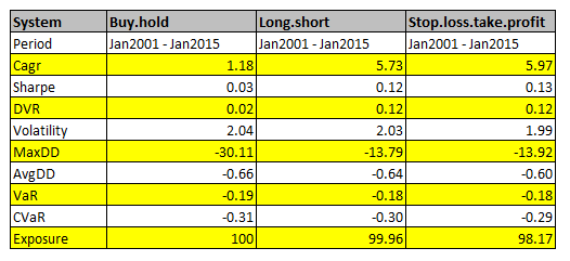
Let us now run all the three models, and check their relative performance.


As you can be seen, the rule-based strategy has a smooth equity curve, and is giving a better CAGR of 5.97 than the simple ‘buy hold’ model CAGR of 1.18. The Maximum drawdown of our strategy is at 13.92 compared to the ‘buy hold’ strategy drawdown of 30.11. You can play with the indicator settings or change the short-long rules or the stop loss-take profit levels to refine the model further.
Once you understand Machine learning algorithms, these can be a great tool for formulating profit-making strategies. To learn more on Machine Learning you can watch our latest webinar, “Machine Learning in Trading”, which was hosted by QuantInsti, and conducted by our guest speaker Tad Slaff, CEO/Co-founder Inovance.
Machine learning is covered in the Executive Programme in Algorithmic Trading (EPAT) course conducted by QuantInsti. If you're looking for a more modular entry point, an algo trading course specifically focused on ML applications in live markets is a great complement to the concepts demonstrated in this post. To know more about EPAT check the EPAT course page or feel free to contact our team at contact@quantinsti.com for queries on EPAT.


