Model a basic trading strategy in python: from idea to execution

By Jacques Joubert

Recently I had the privilege to attend the Python for Quants conference in London via live streaming. Each time I attend this series of lectures I try to capture one of the presentations in writing, this time, I will be writing on a lecture given by Dr. James Munro titled “Quant Strategies: from idea to execution”.

Note that while I have used his lecture for the majority of the information here, I do make changes and add my own experiences. What is written here is not endorsed by Man AHL and use your imagination to add all other disclosures you see fit.

I really enjoyed his lecture as it spoke to me as a professional that spends a lot of time backtesting different strategies. It very nicely captures the common errors in a backtesting.

The course provides valuable insights into backtesting techniques, helping traders identify and avoid common mistakes. With a focus on real-world applications, it enables professionals to refine their strategies and optimize their backtesting process for better performance.

In this article, we cover a rather basic trading strategy, which starts off looking attractive but as we slowly add more realistic factors, you will note how the performance decays.

The strategy is a simple 20 day moving an average crossover strategy. Example: if the current price is above the moving average then buy and hold, else go short and hold. The strategy will be named “ToyStrategy”.

The ToyStrategy will be run on the natural gas futures.

Note that on futures we will have to roll over the contracts and stitch the prices together, which is why we are using the adjusted settlement price.

As a backtesting evangelist, I make a point of spreading the good news of the two different types of frameworks: vectorised and event driven. For this example, Dr. Munro decided on a vectorised backtester which is great for quickly prototyping a strategy but is the greater evil when it comes to accuracy and flexibility.

Steps for a vectorised backtester:

1. Get data (Natural gas)
2. Create your indicator (20 day SMA)
3. Generate signals based on trading logic
4. Generate positions held
5. Calculate performance metrics
6. Plot equity curve

Tada… Here is the first backtest with total returns of $32 million and an information ratio of 2.3.

As most things in life, when someone is trying to sell you something that is too good to be true, it probably is. At first glance, this is an awe-inspiring strategy that should be implemented right away! However, this article will walk you through some of the checks you need to perform in order to validate the strategy.

Step 1: Turn your black box into a glass box

Now there are some strategies that implement machine learning techniques that are harder to turn into a glass box but this is not one of them. The easiest way to improve transparency is to simply plot all of the columns in our data frame.

By doing this we can validate that our model acts as expected.

Chart 1: There are price data available for each day (There are no missing data for very large periods of time).

Chart 2: Clear that the 20 day SMA smooths out the data and that we don’t have any gaps or abnormal spikes.

Chart 3: This signal chart is different to my other backtests as it’s not simply a value where 1 represents a buy, 0 as liquidate, and -1 to go short. In this chart, we have to multiply the signal value by a multiple to generate the Position. (Not the best position sizing technique by a long shot but this is a toy strategy.)

Chart 4: represents the number of lots we are holding at any given point in time.

Chart 5: Daily returns

Step 2: Data Validation

Next, we need to validate that we have clean data. Clean data would include the following checks:

1. Have data for each trading day. If there are data missing then perform a forward fill.
2. Make sure that there are no unrealistic spikes in the data. For example: if the average share price is between 400 and 300 then all of a sudden there is a spike of 4000, you will need to correct this. This also applies to when a value of 0 is inserted into your data.
3. Double check that there are no duplicate dates in your time series
4. Make sure that your data is adjusted for share splits and consolidations, having dividend adjusted prices is a bonus.
5. Beware of free data sources! In my experience, free data sources have less clean data.

Make sure that the data are clean! Personally, a great deal of my time is spent getting and cleaning data. Quandl is said to be a good source and I would agree that Quandl is a good source for free data. However, given the option, I would take a paid source like Bloomberg any day!

Next, we run the following code to check that we have data for each of our trading days and that we can visually see all of our historical positions, this is also part of the glass box concept:

In the screen shot above, you will note that the data only goes up to 2015-11-11 and I know that you can’t tell this from reading the article but I am expecting there to be data up to the 13^th. To correct this Dr. Munro adds a check to his code that allows the ToyStrategy to carry on even if there is some missing data.

This fix is added by stating that the ToyStrategy only needs a minimum of 10 data points to calculate an SMA figure. "min_periods = 10”

Now run the code again and note the nothing has really changed. The ToyStrategy still has the same total return and information ratio as before.

Step 3: Order management and position sizing

Next, you need to validate that the ToyStrategy is implementing the correct position sizing technique and that it is meeting your expectations. In a vectorised backtester this can be a little tricky when dealing with multiple shares but the ToyStrategy is running on just 1 asset and using a vectorised methodology.

In step 2 you will note that the ToyStrategy is using real numbers to represent the number of contracts held at a point in time but this is incorrect, you can only hold an integer number of contracts.

To correct this is simple, just add the round() function.

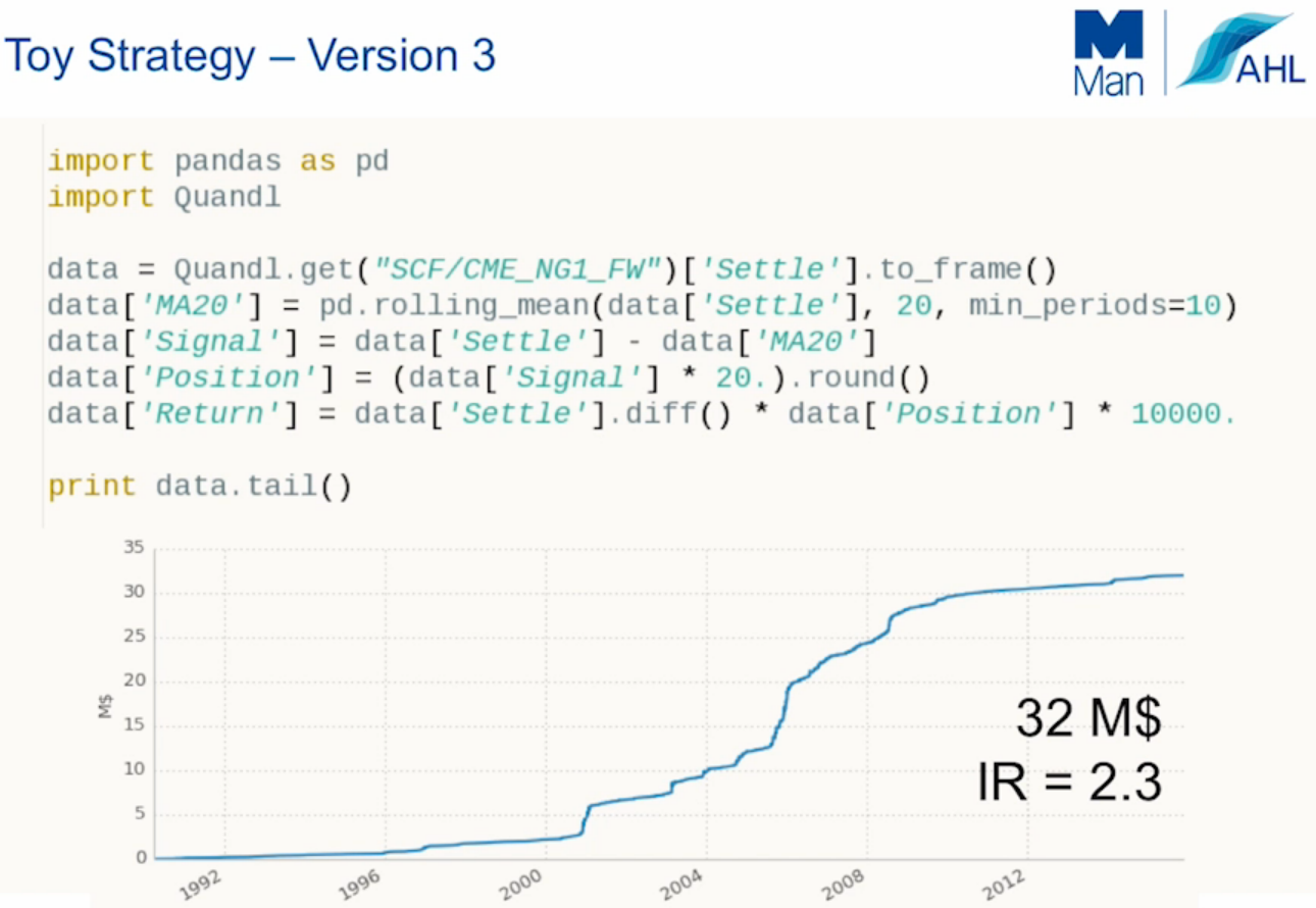
Again nothing has really changed and to double check that we are using whole numbers we run: print data.tail()

Step 4: Make sure you have removed look ahead bias

Next, it is clear that we have to look ahead bias due to the ToyStrategy basing signals on the current day’s closing price. To remedy this we need to lag the data, in this example, we do it by creating a “next position” column and then lagging the values in a new column called Position. In the code below, this is accomplished by adding “.shift(1)”.

Ouch! Here we can see the first major difference in the equity curve. Turns out that the ToyStrategy is less attractive now that it can’t look into the future.

Step 5: Add transaction costs

Up until now, the ToyStrategy strategy has been running without transaction fees and slippage. To add insult to injury, we have to use a very basic method to add the fees because of the vectorised methodology.

A well thought out backtest must include:

• Slippage
• Commissions
• Other liquidity effects
• Position management (risk limits)

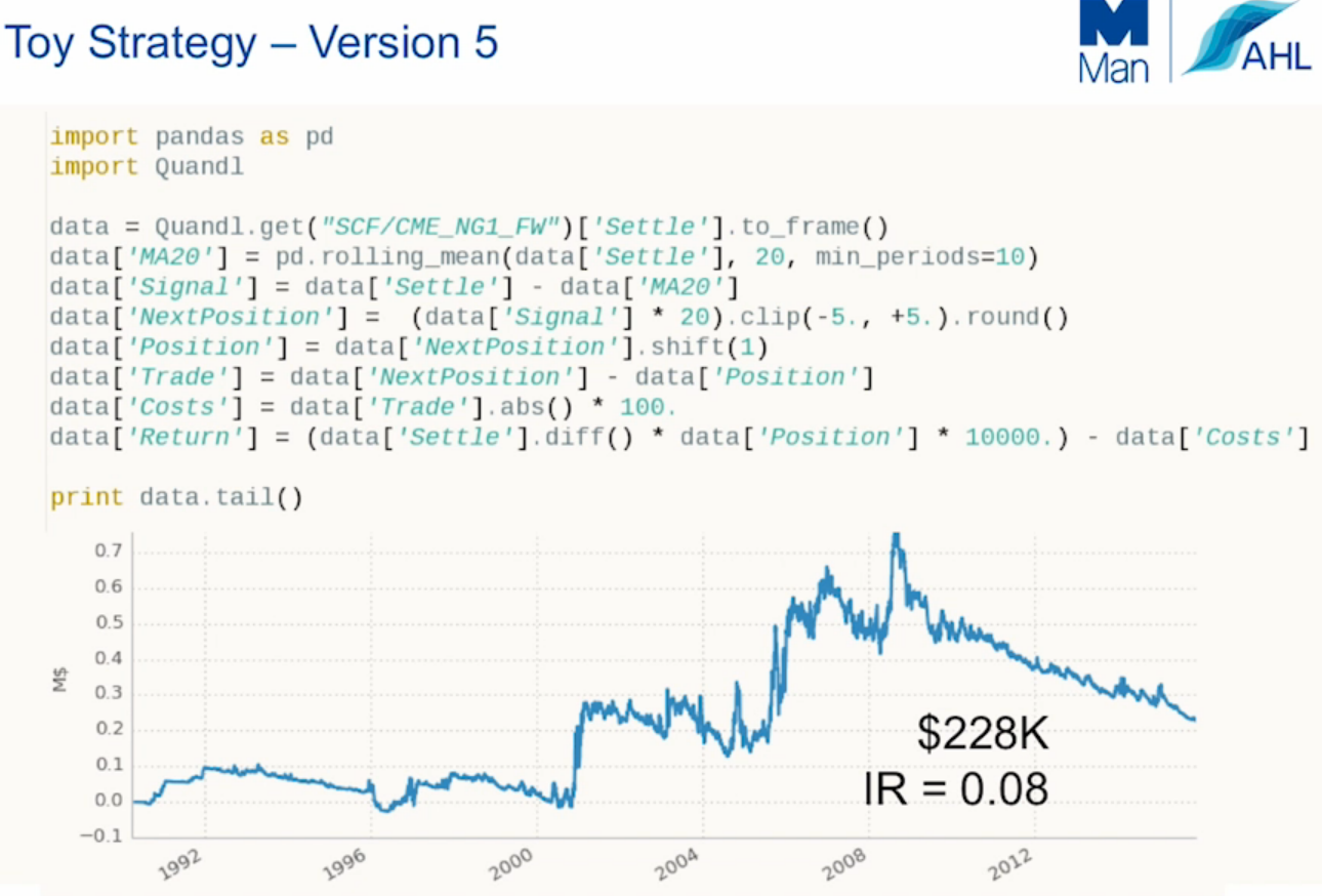
Somehow this strategy is still up, I don’t know how but more importantly we can see that there are no ways that we will be using this strategy going forward.

Step 6: live trading vs. simulation

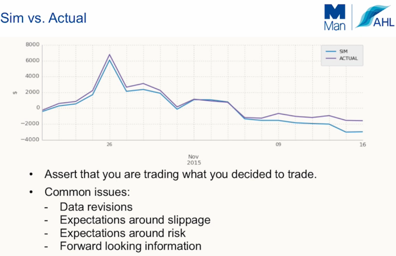
A recommended best practice is to run your simulated results hand in hand with your live trading. By doing this you have a way of searching for errors and fixing bugs.

If you are going to include your simulated results in your fund fact sheet for the public to view then it would be a very good idea to be as prudent as possible. It’s important that you don’t have massive discrepancies between the two. In fact, it’s better if your live results are marginally better than the simulation’s (Better to under promise and over deliver).

Final remarks:

I hope this article has added value to those members of our community that are getting started with backtesting. There are two things that in my experience that make the most dramatic difference, those are:

1. Removing look ahead bias by lagging the signals
2. Adding transaction costs and slippage

If you know of other articles that would help others to get started then please be sure to leave a link in the comments section below.

Next Step

Python algorithmic trading has gained traction in the quant finance community as it makes it easy to build intricate statistical models with ease due to the availability of sufficient scientific libraries like Pandas, NumPy, PyAlgoTrade, Pybacktest and more.

In case you are looking to master the art of using Python to generate trading strategies, backtest, deal with time series, generate trading signals, predictive analysis and much more, you can enroll for our course on Python for Trading!