Neural network studies were started in an effort to map the human brain and understand how humans make decisions but the algorithm tries to remove human emotions altogether from the trading aspect.
What we sometimes fail to realise is that the human brain is quite possibly the most complex machine in this world and has been known to be quite effective at coming to conclusions in record time.
Think about it, if we could harness the way our brain works and apply it in the machine learning domain (Neural networks are after all a subset of machine learning), we could possibly take a giant leap in terms of processing power and computing resources.
Before we dive deep into the nitty-gritty of neural networks for trading, we should understand the working of the principal component, i.e. the neuron and then move forward to the neural network and the applications of neural network in trading.
This blog covers:
A general introduction to neuron
There are three components to a neuron, the dendrites, axon and the main body of the neuron. The dendrites are the receivers of the signal and the axon is the transmitter.
Structure of a Neuron
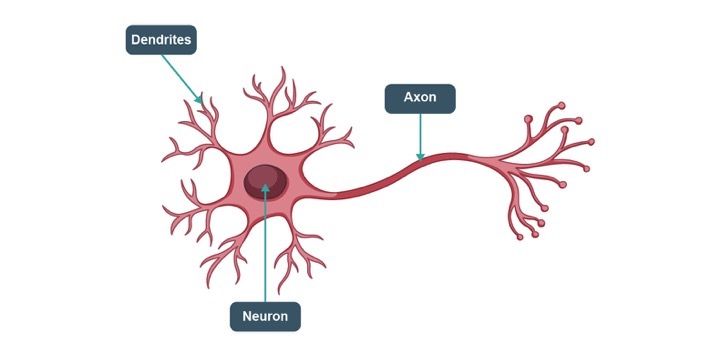
Alone, a neuron is not of much use, but when it is connected to other neurons, it does several complicated computations and helps operate the most complicated machine on our planet, the human body.
You can see in the image below how a group of neurons as inputs lead to an output signal.
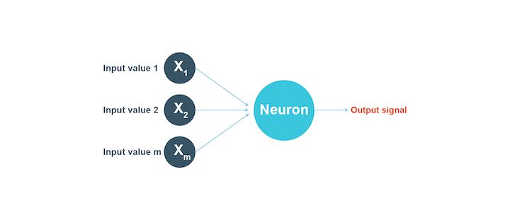
A neural network - An introduction
The neural networks are replicated to work almost like our brain does. Hence, the input layer (it is how humans take inputs from the environment) consists of certain basic information to help arrive at the conclusion or the output.
The output can be to make a prediction, to find out objects of similar characteristics etc. The brain of a human being is filled with senses, such as hearing, touching, smelling, tasting, etc.
The neurons in our brain create complex parameters such as emotions and feelings, from these basic input parameters. And our emotions and feelings, make us act or make decisions which is basically the output of the neural network of our brains. Therefore, there are two layers of computations in this case before making a decision.
Neural Networks in Trading
Additional 27% off
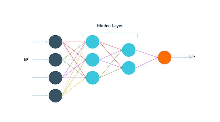
The first layer absorbs the senses as inputs and leads to emotions and feelings as the conclusion. Now, this first layer makes for the inputs of the next layer of computations, where the output is a decision or an action or the final result.
Hence, in the working of the human brain, there is one input layer, two hidden layers, and one output layer leading to a conclusion. The brain is much more complex than just the layers of information, but the general explanation of the computation process of the brain can be defined as such.
Types of neural networks
There are many types of neural networks available. They can be classified depending on a lot of factors. These factors are the data flow, neurons used, their depth and activation filters, the structure, the density of neurons, layers, etc.
Let us see the most common types of neural networks (neural network trading), and these are:
- Perceptron
- Feed forward neural networks
- Multilayer perceptron
- Convolutional neural network
- Recurrent neural network
- Modular neural network
Perceptron

Perceptron belongs to the supervised learning algorithm. As you can see in the image above, the data is split into two categories. Hence, perceptron is a binary classifier.
The Perceptron model is known to be the smallest unit of the neural network. Perceptron works to find out the features of the input data. The Perceptron model works with the weights as the inputs and also applies an activation function. This way the final result comes about.
Feed Forward neural networks
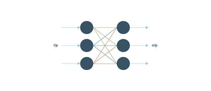
The feed-forward neural network is quite simple since its input data passes through the artificial neural nodes or input nodes and exits through the output nodes. This implies that the data travels in one direction and the information in depth is not available.
The feed forward neural network is a unidirectional forward propagation with no backpropagation. The weights are static in this type and the activation function has inputs that are multiplied by the weights. For the feed forward to work, a classifying activation function is used.
Let us understand the concept of forward feed with an example. For example,
- Output of neuron is above threshold (0), i.e., is 1 - This implies that the neuron is activated
- Output of neuron at the threshold (0) or is below threshold (-1) - This implies that the neuron is not activated
The best thing about the feed forward neural network is that it can deal with a lot of noise in the data.
Multilayer perceptron
A multilayer perceptron does what its name suggests. The input data, in the case of a multilayer perceptron, goes through a lot of layers of artificial neurons. Hence, the input and output layers consist of multiple layers with a lot of information regarding the input. Each node in this type is connected with the neurons in the next layer.
The multilayer perceptron is known to be the fully connected one. Also, this type has a bi-directional propagation, which implies forward propagation as well as backpropagation.
The multilayer perceptron works by multiplying the inputs with the weights and the result is given to the activation function. On the other hand, in backpropagation, the result is modified in order to reduce the losses.
Convolutional neural network
The convolutional neural network consists of a three-dimensional structure of neurons and not the two-dimensional one. It works in the following way:
- The first layer is known as the convolutional layer.
- Each neuron in the convolutional layer takes into consideration only a small part of the information in the data in order to include more details.
- The input pointers are in a batch.
- The neural network processes all the inputs in images.
- Each image is learnt by a neural network in parts.
- The operations are computed several times to complete the processing of the image.
- The image is converted from a particular scale and then the image is classified into several categories.
In this type, the propagation is unidirectional and the neural network consists of one or more convolutional layers. The bidirectional version of this type makes the output of the convolutional layer go to a fully connected neural network. Also, the filters are used for extracting the parts of the image.

In this type, the inputs are multiplied with weights and used by the activation function.
Recurrent neural networks
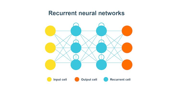
Recurrent neural network or RNN is quite helpful in modelling sequenced data from the start to the end.
In this type of neural network, the first layer, as represented by the yellow coloured cells, is basically the feed-forward neural network. The second layer is the recurrent neural network layer where the information fed to it in the first layer is memorised. This is the forward propagation.
Now, the information is fed for use in the future and is corrected until the prediction made is as expected. This time the backpropagation occurs to make it to the correct information.
Modular neural network
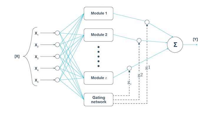
In the case of the modular neural network, several neural networks work independently to perform small tasks leading to the main task. While the modular neural network works, the different networks do not interact at all. This increases efficiency as each network works towards the same goal.
Just like humans, when several neural networks work together with each working on a sub-task, the complex or large process is completed faster. The independent components ensure that each piece of information is provided in detail to lead to the final conclusion.
How to train a neural network?
To simplify things in the neural network tutorial, we can say that there are two ways to code a program for performing a specific task.
- All the rules of the program are to be defined. Also, the inputs will be given to the program in order to compute the result.
- Develop the framework upon which the code will learn to perform the specific task by training itself on a dataset by adjusting the result it computes to be as close to the actual results which have been observed.
The second process is called training the model which is what we will be focussing on. Let’s look at how our neural network will train to predict stock prices.
The neural network will be given the dataset, which consists of the OHLCV data as the input, as well as the output, we would also give the model the Close price of the next day, this is the value that we want our model to learn to predict. The actual value of the output will be represented by ‘y’ and the predicted value will be represented by y^ (y hat).
The model's training involves adjusting the variables' weights for all the different neurons present in the neural network. This is done by minimising the ‘Cost Function’. The cost function, as the name suggests, is the cost of making a prediction using the neural network. It is a measure of how far off the predicted value, y^, is from the actual or observed value, y.
There are many cost functions that are used in practice, the most popular one is computed as half of the sum of squared differences between the actual and predicted values for the training dataset.
$$ C = \sum 1/2 (y^^-y)^2 $$The neural network, first of all, trains itself by computing the cost function for the training dataset. Also, it is important to note that the training dataset holds a given set of weights for the neurons. Afterwards, the neural network tries to improve itself by going back and adjusting the weights.
Then it computes the cost function for the new training dates with the new weights. This entire process of the correction of the errors and adjusting of the weights after corrections are known as backpropagation.
The cost function is to be minimised and this backpropagation is repeated till the cost function is minimised. Here, the weights are also adjusted.
One way to do this is through brute force. Let us assume that there are 1000 values for the weights. Now, we will evaluate the cost function with these 1000 values.
The graph of the cost function will look like the one below.
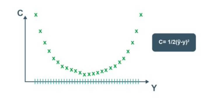
This approach could be successful for a neural network involving a single weight which needs to be optimised. However, as the number of weights to be adjusted and the number of hidden layers increases, the number of computations required will increase drastically.
The time it will require to train such a model will be extremely large even on the world’s fastest supercomputer. For this reason, it is essential to develop a better, faster methodology for computing the weights of the neural network. This process is called Gradient Descent.
Gradient descent
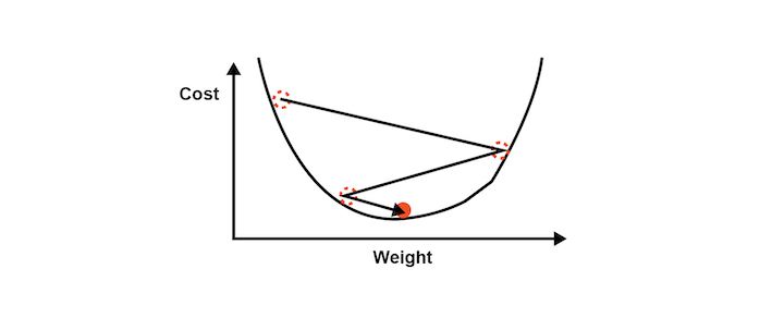
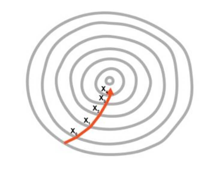
Gradient descent analyses the cost function and it shows via the slope of the curve as shown in the image below. Based on the slope we adjust the weights. This helps to minimise the cost function.
The visualisation of Gradient descent is shown in the diagrams below. The first plot is two dimensional. The image below shows the red circle moving in a zig-zag pattern to reach the minimum cost function eventually.
In the second image, the adjustment of two weights is needed in order to minimise the cost function.
Hence, it can be seen as a contour in the image where the direction is toward the steepest slope and the minimum is to be reached in the shortest time period. This approach does not require a lot of computational processes and the process is not extremely lengthy either. You can say that the training of the model is a feasible task.
Gradient descent can be done in three possible ways,
- Batch gradient descent
- Stochastic gradient descent
- Mini-batch gradient descent
Batch gradient descent
The batch gradient descent is the one in which the cost function is calculated by finding out the sum of all individual cost functions in the training dataset. After this step, the slope is computed by adjusting the weights of the training dataset.
Stochastic gradient descent
In this type of gradient descent, each data entry is followed by the creation of slope of the cost function and the adjustment of the weights in the training dataset. This helps to avoid the local minima if the cost function curve is not convex.
Also, each time the stochastic gradient descent’s process to reach the minimum will appear different.
Mini-batch gradient descent
The third type is the mini-batch gradient descent, which is a combination of batch and stochastic methods. Here, we create different batches by clubbing together multiple data entries in one batch. This essentially results in implementing the stochastic gradient descent on bigger batches of data entries in the training dataset.
While we can dive deep into Gradient Descent, we are afraid it will be outside the scope of the neural network tutorial. Hence let’s move forward and understand how backpropagation works to adjust the weights according to the error which had been generated.
Backpropagation
Backpropagation is an advanced algorithm which enables us to update all the weights in the neural network simultaneously. This drastically reduces the complexity of the process to adjust weights. If we were not using this algorithm, we would have to adjust each weight individually by figuring out what impact that particular weight has on the error in the prediction.
Let us look at the steps involved in training the neural network with Stochastic Gradient Descent:
- Step 1 - Initialise the weights to small numbers. The number should be very close to 0 (but not 0)
- Step 2 - Forward propagation - The neurons are activated from left to right, by using the first data entry in our training dataset, until we arrive at the predicted result y
- Step 3 - Error Computation - Measure the error which will be generated
- Step 4 - Backpropagation - The error generated will be back propagated from right to left. Also, the weights will be adjusted according to the learning rate
- Step 5 - Repeat the previous three steps. The three steps of forward propagation, error computation and backpropagation will go through the entire training dataset
- Step 6 - This would mark the end of the first epoch. The successive epochs will begin with the weight values of the previous epochs, Now, we can stop this process when the cost function reaches an acceptable limit
We have covered a lot in this neural network tutorial and this leads us to apply these concepts in practice. Thus, we will now learn how to develop our own Artificial Neural Network (ANN) to predict the movement of a stock price.
You will understand how to code a strategy using the predictions from a neural network that we will build from scratch. You will also learn how to code the Artificial Neural Network in Python, making use of powerful libraries for building a robust trading model using the power of neural networks.
Neural network in trading
Neural networks help you develop strategies based on your overall investment strategy ⁽¹⁾. Whether it is high-risk and growth-focused (short-term trades) or a conservative approach for long-term investment, it all depends on the kind of trading strategy.
For example, you wish to find a few stocks with particular growth performance or an upward price trend over a period of one year. Now, the neural network can figure out such stocks for your portfolio and hence, make your work easy.
Also, you can give a number of such parameters or necessary pointers to the neural network so that you have exactly what you are looking for with less effort and time.
Neural network strategy in Python
Let us now see the strategical representation with neural networks in Python.
First of all we will import libraries.
Step 1: Importing Libraries
We will start by importing a few libraries, the others will be imported as and when they are used in the program at different stages. For now, we will import the libraries which will help us in importing and preparing the dataset for training and testing the model.
Numpy is a fundamental package for scientific computing, we will be using this library for computations on our dataset. The library is imported using the alias np.
Pandas will help us in using the powerful dataframe object, which will be used throughout the code for building the artificial neural network in Python.
Ta-lib is a technical analysis library, which will be used to compute the RSI and Williams %R. These will be used as features in order to train our artificial neural network or ANN. We could add more features using this particular library, and many courses for technical analysis teach how to effectively use such libraries for market analysis.
Step 2: Fetching data from yahoo finance
Random is used to initialise the seed to a fixed number. This is such that every time we run the code we start with the same seed.
We have taken Apple’s data for the time period 6th November 2017 to 3rd January 2023.
Step 3: Preparing the dataset
We will be building our input features by using only the OHLC values. This dataset will help us to specify the features for training our neural network in the next step.
Step 4: Defining input features from dataset
We then prepare the various input features which will be used by the artificial neural network learning for making the predictions. We define the following input features:
- High minus Low price
- Close minus Open price
- Three day moving average
- Ten day moving average
- 30 day moving average
- Standard deviation for a period of 5 days
- Relative Strength Index
- Williams %R
We then define the output value as price rise, which is a binary variable storing 1 when the closing price of tomorrow is greater than the closing price of today.
Next, we drop all the rows storing NaN values by using the dropna() function.
We then create two data frames to store the input and the output variables. The dataframe ‘x’ stores the input features. The columns start from the fifth column of the dataset and go on to the second last column. The last column will be stored in the dataframe ‘y’ (prediction value) which is the rise in the prices.
In this part of the code, we will split our input and output variables to create the test and train datasets. This is done by creating a variable called split, which is defined to be the integer value of 0.8 times the length of the dataset.
We then slice the X and y variables into four separate data frames: Xtrain, Xtest, ytrain and ytest. This is an essential part of any machine learning algorithm, the training data is used by the model to arrive at the weights of the model.
The test dataset is used to see how the model will perform on new data which would be fed into the model. The test dataset also has the actual value for the output, which helps us in understanding how efficient the model is.
We will look at the confusion matrix later in the code, which essentially is a measure of how accurate the predictions made by the model are.
Step 5: Standardise the dataset (Data preprocessing)
Another important step in data preprocessing is to standardise the dataset. This process makes the mean of all the input features equal to zero and also converts their variance to 1. This ensures that there is no bias while training the model due to the different scales of all input features.
If this is not done the neural network might get confused and give a higher weight to those features which have a higher average value than others.
We implement this step by importing the StandardScaler method from sklearn.preprocessing library. We instantiate the variable sc with the StandardScaler() function.
Step 6: Building the artificial neural network model
After this we use the fittransform function to implement these changes on the Xtrain and Xtest datasets. The ytrain and y_test sets contain binary values, hence they need not be standardised. Now that the datasets are ready, we may proceed with building the Artificial Neural Network using the Keras library.
Now we will import the functions which will be used to build the artificial neural network. We import the Sequential method from the keras.models library. This will be used to sequentially build the layers of the neural networks learning. The next method that we import will be the Dense function from the keras.layers library.
This method will be used to build the layers of our artificial neural network.
We instantiate the Sequential() function into the variable classifier. This variable will then be used to build the layers of the artificial neural network learning in Python.
To add layers to our Classifier, we make use of the add() function. The argument of the add function is the Dense() function, which in turn has the following arguments:
- Units: This defines the number of nodes or neurons in that particular layer. We have set this value to 128, meaning there will be 128 neurons in our hidden layer.
- Kernel_initializer: This defines the starting values for the weights of the different neurons in the hidden layer. We have defined this to be ‘uniform’, which means that the weights will be initialised with values from a uniform distribution.
- Activation: This is the activation function for the neurons in the particular hidden layer. Here we define the function as the rectified Linear Unit function or ‘relu’.
- Input_dim: This defines the number of inputs to the hidden layer, we have defined this value to be equal to the number of columns of our input feature dataframe. This argument will not be required in the subsequent layers, as the model will know how many outputs the previous layer produced.
We then add a second layer, with 128 neurons, with a uniform kernel initializer and ‘relu’ as its activation function. We are only building two hidden layers in this neural network.
The next layer that we build will be the output layer, from which we require a single output. Therefore, the units passed are 1, and the activation function is chosen to be the Sigmoid function because we would want the prediction to be a probability of the market moving upwards.
Finally, we compile the classifier by passing the following arguments:
- Optimizer: The optimizer is chosen to be ‘adam’, which is an extension of the stochastic gradient descent.
- Loss: This defines the loss to be optimised during the training period. We define this loss to be the mean squared error.
- Metrics: This defines the list of metrics to be evaluated by the model during the testing and training phase. We have chosen accuracy as our evaluation metric.
Now we need to fit the neural network that we have created to our train datasets. This is done by passing Xtrain, ytrain, batch size and the number of epochs in the fit() function.
The batch size refers to the number of data points that the model uses to compute the error before backpropagating the errors and making modifications to the weights. The number of epochs represents the number of times the training of the model will be performed on the train dataset.
Step 7: Setting the prediction parameters
With this, our artificial neural network in Python has been compiled and is ready to make predictions.
Now that the neural network has been compiled, we can use the predict() method for making the prediction. We pass X_test as its argument and store the result in a variable named ypred. We then convert ypred to store binary values by storing the condition ypred >0.5. Now, the variable y_pred stores either True or False depending on whether the predicted value was greater or less than 0.5.
Next, we create a new column in the dataframe dataset with the column header ‘y_pred’ and store NaN values in the column. We then store the values of y_pred in this new column, starting from the rows of the test dataset.
This is done by slicing the dataframe using the iloc method as shown in the code above. We then drop all the NaN values from the dataset and store them in a new dataframe named trade_price_AAPL.
Step 8: Computation of strategy returns and determine trade positions
Now that we have the predicted values of the stock movement. We can compute the returns of the strategy. We will be taking a long position when the predicted value of y is true and will take a short position when the predicted signal is False.
We first compute the returns that the strategy will earn if a long position is taken at the end of today and squared off at the end of the next day. We start by creating a new column named ‘Tomorrows Returns’ in the trade_price_AAPL and store in it a value of 0.
We use decimal notation to indicate that floating point values will be stored in this new column. Next, we store in it the log returns of today, i.e. logarithm of the closing price of today divided by the closing price of yesterday. Next, we shift these values upwards by one element so that tomorrow’s returns are stored against the prices of today.
Next, we will compute the strategy returns. We create a new column under the header ‘StrategyReturns’ and initialise it with a value of 0 to indicate storing floating point values.
By using the np.where() function, we then store the value in the column ‘Tomorrows Returns’ if the value in the ‘ypred’ column stores True (a long position), else we would store the negative of the value in the column ‘Tomorrows Returns’ (a short position); into the ‘Strategy Returns’ column.
We now compute the cumulative returns for both the market and the strategy. These values are computed using the cumsum() function. We will use the cumulative sum to plot the graph of market and strategy returns in the last step.
We will now plot the market returns and our strategy returns to visualise how our strategy is performing against the market. For this, we will import matplotlib.pyplot.
We then use the plot function to plot the graphs of Market Returns and Strategy Returns using the cumulative values stored in the dataframe trade_dataset. We then create the legend and show the plot using the legend() and show() functions respectively.
The plot shown below is the output of the code. The green line represents the returns generated using the strategy and the red line represents the market returns.
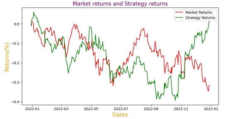
You can see in the output above that the strategy returns peaked in Jan, 2023 after fluctuating (upwards and downwards) throughout the other time periods.
The strategy returns are seen outperforming the market returns as well occasionally.
Similarly, you can modify the strategy parameters according to your understanding of the market and expectations.
Conclusion
With the blog coming to an end, we believe that you can now build your own Artificial Neural Network in Python and start trading using the power and intelligence of your machines.
Apart from Neural Networks, there are many other machine learning models that can be used for trading. The Artificial Neural Network or any other Deep Learning model will be most effective when you have more than 100,000 data points for training the model.
Artificial intelligence in trading has become pivotal for real-time data processing and strategic analysis. By using AI, platforms can interpret market sentiments and respond to emerging patterns faster than traditional methods, enhancing the effectiveness of trading decisions and risk management.
This model was developed on daily prices to make you understand how to build the model. It is advisable to use the minute or tick data for training the model, which will give you enough data for effective training.
You can enrol in the neural network course on Quantra where you can use advanced neural network techniques and the latest research models such as LSTM & RNN to predict markets and find trading opportunities. Keras, the relevant Python library is used.
Bibliography
Srinath R1, Sarvaesh Raam S2, May 2022
Note: The original post has been revamped on 11th May 2023 for accuracy, and recentness.
Disclaimer: All data and information provided in this article are for informational purposes only. QuantInsti® makes no representations as to accuracy, completeness, currentness, suitability, or validity of any information in this article and will not be liable for any errors, omissions, or delays in this information or any losses, injuries, or damages arising from its display or use. All information is provided on an as-is basis.


