Portfolio Allocation and Pair Trading Strategy using Python

Learn to perform a comparative analysis of the Portfolio Allocation Strategy with the Pair trading strategy, using the Sharpe, Sortino and Calmar ratio.

The complete data files and python code used in this project are available in a downloadable format at the end of the article.

This article is the final project submitted by the author as a part of his coursework in Executive Programme in Algorithmic Trading (EPAT) at QuantInsti. Do check our Projects page and have a look at what our students are building.

About the Author

Ravindra Singh Rawat has a Bachelors’ degree in Electronics and Telecommunication Engineering from NMIMS University. Previously, he has worked with Talerang (a company incubated at Harvard) and QuantInsti. He has a keen interest in analyzing financial data and he aspires to build a career in the financial markets in some capacity.

Project Abstract

The aim of the project is to compare the Portfolio Allocation Strategy with the Pair trading strategy.

The scope of the project is the Indian Equities Market.Our aim was to perform a comparative analysis using the Sharpe, Sortino and Calmar ratio.

• Under the above assumptions, it was found that Allocation works better for the following sectors: Pharmaceuticals and Financial Services basket.
• Pairs Trading seems to be a better alternative for the following sectors: Technology, Automobile, and Private Banks basket.

It is advisable to use the Sharpe ratio metric along with the Sortino and Calmar ratio metrics, as the latter two ratios take into account the downside risk and the drawdown associated with a particular strategy.

A brief history of the Ratios

The Sharpe Ratio was developed after William F. Sharpe in 1966.  It measures the performance of an investment (e.g., security or portfolio) compared to a risk-free asset, after adjusting for its risk.

One of the key criticisms of the Sharpe Ratio was that it was poor at estimating tail risks; a normal distribution is assumed, hence it cannot differentiate between positive and negative trades.

This gave rise to the Post Modern Portfolio Theory. The post-modern portfolio theory (PMPT) is a portfolio optimization methodology that uses the downside risk of returns instead of the mean variance of investment returns used by the Modern Portfolio Theory (MPT) i.e the Sortino Ratio.

The PMPT stands in contrast to the modern portfolio theory (MPT); both of which detail how risky assets should be valued while stressing the benefits of diversification, with the difference in the theories being how they define risk and its impact on returns.

Brian M. Rom and Kathleen Ferguson, two software designers, created the PMPT in 1991 when they believed there to be flaws in software design using the MPT.

The year 1991 also gave rise to the Calmar Ratio. It was created by Terry W. Young and first published in the trade journal titled ‘Futures’.  Young owned California Managed Accounts, a firm in Santa Ynez, California, which managed client funds and published the newsletter CMA Reports. The name of his ratio "Calmar" is an acronym of his company's name and his newsletter:

CALifornia Managed Accounts Reports

Young defined it thus:

"The Calmar ratio is the average annual rate of return for the last 36 months divided by the maximum drawdown for the last 36 months. It is calculated on a monthly basis."

Young believed the Calmar ratio was superior because:

The Calmar ratio changes gradually and serves to smooth out the overachievement and underachievement periods of a CTA's (Commodity Trading Advisors) performance more readily than the Sharpe ratio.

Ideation

The first time that I came across the phrase ‘Monte Carlo simulations’ was when I was reading the book titled ‘Fooled by Randomness’ by Nassim Nicholas Taleb. I found the idea of running multiple simulations to be very intriguing.

While I was learning about the Pair Trading Strategy during my EPAT sessions, I thought to myself, why not create a project where I compare the Portfolio Allocation (Monte Carlo simulation based) strategy to a Pair trading strategy. Right then and there I had my project idea.

Project Description

My idea was simple: I wanted to compare a Portfolio Allocation strategy with a Pair Trading (using Mean Reversion) strategy.

In fact, I used a triplet i.e 3 stocks instead of a pair, for both the strategies. The basis on which I would compare the effectiveness of the said strategies would be based on the following ratios:

• Sharpe
• Sortino
• Calmar

Sharpe Ratio

It is the ratio for comparing reward (return on investment) to risk (standard deviation). This allows us to adjust the returns on an investment by the amount of risk that was taken in order to achieve it.

This is given by the following formula:

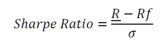
• 𝑅 - annual expected return of the asset in question.
• 𝑅𝑓 - annual risk-free rate. Think of this as a deposit in the bank earning x% per annum.
• 𝜎 - annualized standard deviation of returns

Sortino Ratio

The Sortino ratio is very similar to the Sharpe ratio, the only difference being that where the Sharpe ratio uses all the observations for calculating the standard deviation,  the Sortino ratio only considers the negative variance.

The rationale for this is that we aren't too worried about positive deviations, however, the negative deviations are of great concern, since they represent a loss of our money. This is given by the following formula:

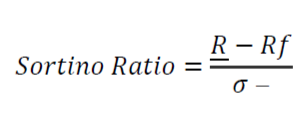
• R - annual expected return of the asset in question.
• 𝑅𝑓 - annual risk-free rate.
• 𝜎 - annualized downside standard deviation of returns

Calmar ratio

This is similar to the other ratios, with the key difference being that the Calmar ratio uses max drawdown in the denominator as opposed to standard deviation.

• R -  annual expected return of the asset in question.
• 𝑅𝑓 - annual risk-free rate.

For the purpose of my project, I have considered Rf to be 0, for all ratios.

I collected the data from the Yahoo Finance website. The data was pertaining to stocks in the Indian stock market. The stock data was dated from 29th May 2017 to 30th June 2020. The sectors that I have compared are Technology, Finance(Private Banks), Finance(Financial Services), Automobile, and Pharma. From each sector, I have selected 3 stocks at random.

Portfolio Allocation Strategy methodology

At first, I computed the Sharpe ratio. The procedure was as follows:

• I imported the relevant stock data from Yahoo Finance.
• Then I calculated the Return of the Adjusted Close prices using the pct_change() method.
• After that, I calculated the mean of returns and the covariance matrix. The covariance matrix tells us about the relationship between the movement of 2 stocks.
• In order to run a simulation, I first had to create a matrix. Since I planned to run 10000 simulations, I initialized the rows to be of the number 10000. In the said matrix, I wanted to display the Mean returns, Standard deviation, Sharpe ratio, and the 3 stocks. Hence the matrix would be of the order 10000 x 6
• The 3 ‘stocks’ columns would display their respective weightage in the portfolio. The idea was to randomize the weightage of the stocks in the portfolio (The weights are assigned inside a 'for loop').
• Initially, all the values in the matrix are displayed as zero because no values are fed to it.
• The main computation takes place inside the 'for loop'.
• Portfolio return is calculated as follows:

𝑃𝑜𝑟𝑡𝑓𝑜𝑙𝑖𝑜 𝑟𝑒𝑡𝑢𝑟𝑛=𝑀𝑒𝑎𝑛 𝑟𝑒𝑡𝑢𝑟𝑛𝑠∗𝑤𝑒𝑖𝑔ℎ𝑡𝑠∗252

Where 252 is the number of trading days in a year

• Portfolio Standard deviation is calculated as follows:

𝑃𝑜𝑟𝑡𝑓𝑜𝑙𝑖𝑜 𝑆𝑡𝑎𝑛𝑑𝑎𝑟𝑑 𝑑𝑒𝑣𝑖𝑎𝑡𝑖𝑜𝑛= √(𝑤𝑒𝑖𝑔ℎ𝑡𝑠)∙((√𝐶𝑜𝑣𝑎𝑟𝑖𝑎𝑛𝑐𝑒 𝑀𝑎𝑡𝑟𝑖𝑥)∙(√𝑤𝑒𝑖𝑔ℎ𝑡𝑠))

The Portfolio Standard deviation is the square root of the dot product of weights and dot product of Covariance matrix and weights.

• Then we calculate the Sharpe ratio by dividing the portfolio return by the Portfolio Standard deviation.

𝑆ℎ𝑎𝑟𝑝𝑒 𝑟𝑎𝑡𝑖𝑜= 𝑃𝑜𝑟𝑡𝑓𝑜𝑙𝑖𝑜 𝑟𝑒𝑡𝑢𝑟𝑛/𝑃𝑜𝑟𝑡𝑓𝑜𝑙𝑖𝑜 𝑆𝑡𝑎𝑛𝑑𝑎𝑟𝑑 𝑑𝑒𝑣𝑖𝑎𝑡𝑖𝑜𝑛

• We then populate the ‘zero’ matrix with the required values.
• Our aim is to find the following portfolios: One with the maximum Sharpe ratio and the other with the least Standard deviation.
• For that we use the ‘iloc’ functionality of pandas, to locate the following rows.
• The ‘iloc’ functionality is used in conjunction with ‘idxmax’ and ‘idxmin’ functionalities to compute the portfolios with the maximum Sharpe ratio and the least Standard deviation respectively.
• At the end, we plot our results using the matplotlib library.

Procedure for computing the Sortino ratio

• The procedure is similar to calculating the Sharpe ratio. The difference lies in the for loop i.e the calculations inside it
• First I calculated the daily portfolio return
• Then I calculated the mean of the portfolio return (using the mean() method ) and multiplied it by 252, in order to annualize the return.
• In order to calculate the downside Standard deviation, I only considered those Portfolio returns which were negative (using the np.where method as a filter). The Standard deviation was calculated using the std() method.
• After that I calculate the Sortino ratio:

𝑆𝑜𝑟𝑡𝑖𝑛𝑜 𝑅𝑎𝑡𝑖𝑜= 𝐴𝑛𝑛𝑢𝑎𝑙𝑖𝑠𝑒𝑑 𝑃𝑜𝑟𝑡𝑓𝑜𝑙𝑖𝑜 𝑟𝑒𝑡𝑢𝑟𝑛/𝐷𝑜𝑤𝑛𝑠𝑖𝑑𝑒 𝑆𝑡𝑎𝑛𝑑𝑎𝑟𝑑 𝑑𝑒𝑣𝑖𝑎𝑡𝑖𝑜𝑛

• After using the ‘iloc’ functionality as I had done whilst calculating the Sharpe ratio, I plotted the results using the matplotlib library.

Procedure for calculating the Calmar ratio

• The procedure is similar to calculating the Sharpe ratio. The difference lies in the for loop i.e the calculations inside it
• First I calculated the daily portfolio return
• After that, I created a function called maximum drawdown. This function is used to calculate the drawdown as follows:

𝐷𝑟𝑎𝑤𝑑𝑜𝑤𝑛= 1−(𝑃𝑜𝑟𝑡𝑓𝑜𝑙𝑖𝑜 𝑟𝑒𝑡𝑢𝑟𝑛.𝑅𝑢𝑛𝑛𝑖𝑛𝑔 𝑀𝑎𝑥)

• Portfolio return can be thought of as equity and running max as Peak drawdown equity. Running Max is always greater than or equal to Portfolio return.
• After that, I computed the maximum drawdown using the max() function
• Once this was done, I proceeded to calculate the Calmar Ratio as follows:

𝐶𝑎𝑙𝑚𝑎𝑟 𝑟𝑎𝑡𝑖𝑜= 𝑃𝑜𝑟𝑡𝑓𝑜𝑙𝑖𝑜 𝑟𝑒𝑡𝑢𝑟𝑛/𝑀𝑎𝑥𝑖𝑚𝑢𝑚 𝐷𝑟𝑎𝑤𝑑𝑜𝑤𝑛

• After using the ‘iloc’ functionality as I had done whilst calculating the Sharpe ratio, I plotted the results using the matplotlib library.

Procedure for the Pair trading strategy

At first, I imported the data from Yahoo finance.

• Unlike the Portfolio Allocation strategy, I am only interested in the price series. Hence I only imported the Adjusted Close series and did not calculate the return.

After that, I plotted the series using the plot() method.

• Now we get into the nitty-gritty of the pair trading strategy. I started by calculating the hedge ratio.
• The Hedge ratio tells us about the number of shares we have to buy/sell for the strategy to remain mean reverting.
  For e.g.  I buy a share of  X, and the hedge ratio for Y is 1.29 and for Z is -2.29. This means that when I buy a share of X, I need to sell 1.29 shares of Y and buy 2.29 shares of Z for the strategy to remain mean reverting.

Then I calculated the spread of the strategy. The spread is the difference between the long position and the short position.

Then I plotted the spread.

• For a pair trading strategy, the spread must be stationary. To check this, we perform a statistical test called the ADF test.
• To satisfy the ADF test, the P-value at ADF index 0 i.eADF[0] must be less than the P- values at ADF index 4 i.e ADF[4].

After that, I created a function called ‘stat_arb’ and the values fed to it were the Adjusted Close price, the lookback period and the Standard deviation.

• The ‘stat_arb’ was created so that I could generate signals for the pair trading strategy. The signals are generated using Bollinger bands. The Bollinger band consists of 3 lines: the moving average, lower band and upper band.
• Inside the function, I calculated the Moving Average and the Moving Standard Deviation. Lookback was used as a value for the rolling window.

Then I computed the Upper band and the Lower band:

Upper Band = Moving Average + Standard Deviation * Moving Standard Deviation

Lower Band = Moving Average - Standard Deviation * Moving Standard Deviation

Then I created the entry and exit positions for the long and short positions.

• A long entry is when the spread is lesser than the lower band.
• A long exit is when the spread is greater than or equal to the moving average.
• A short entry is when the spread is greater than the upper band.
• A short exit is when the spread is lesser than or equal to the moving average.
• An exit is denoted by 0. Along entry is denoted by 1 and a short entry is denoted by -1.
• A net position is the summation of long and short positions.

Then I calculated the spread difference so that I could calculate the pnl. The spread difference is Today’s spread – The previous day’s spread. The pnl is the spread difference multiplied by the net positions. The net position is shifted by 1 i.e the previous day, in order to avoid the look-ahead bias.

After that, I calculated the cumulative pnl. The strategy returns are needed to calculate the Sharpe, Sortino and Calmar ratio. To calculate the strategy returns I first need to calculate the percentage change of spread.

𝑃𝑒𝑟𝑐𝑒𝑛𝑡𝑎𝑔𝑒 𝑐ℎ𝑎𝑛𝑔𝑒 𝑜𝑓 𝑠𝑝𝑟𝑒𝑎𝑑=(𝑇𝑜𝑑𝑎𝑦′𝑠𝑝𝑟𝑒𝑎𝑑−𝑃𝑟𝑒𝑣𝑖𝑜𝑢𝑠 𝑑𝑎𝑦′𝑠 𝑠𝑝𝑟𝑒𝑎𝑑)/( 𝑝𝑎𝑟𝑎𝑚𝑒𝑡𝑒𝑟 0∗𝐴𝑑𝑗𝑢𝑠𝑡𝑒𝑑 𝐶𝑙𝑜𝑠𝑒 𝑜𝑓 𝑆𝑡𝑜𝑐𝑘 𝐵∗𝑆ℎ𝑖𝑓𝑡(1)+(𝑝𝑎𝑟𝑎𝑚𝑒𝑡𝑒𝑟 0∗𝐴𝑑𝑗𝑢𝑠𝑡𝑒𝑑 𝐶𝑙𝑜𝑠𝑒 𝑜𝑓 𝑆𝑡𝑜𝑐𝑘 𝐶∗𝑆ℎ𝑖𝑓𝑡(1)+𝑆𝑡𝑜𝑐𝑘 𝐴

𝑆𝑡𝑟𝑎𝑡𝑒𝑔𝑦 𝑟𝑒𝑡𝑢𝑟𝑛𝑠=𝑛𝑒𝑡 𝑝𝑜𝑠𝑖𝑡𝑖𝑜𝑛.𝑠ℎ𝑖𝑓𝑡(1)∗𝑝𝑒𝑟𝑐𝑒𝑛𝑡𝑎𝑔𝑒 𝑐ℎ𝑎𝑛𝑔𝑒 𝑜𝑓 𝑠𝑝𝑟𝑒𝑎𝑑

The net position is shifted by a day to avoid look-ahead bias.

Then I calculated the cumulative product of strategy returns (cumulative returns) and plotted it on a graph. In another cell, I plotted the cumulative returns with the

Then I proceeded with calculating the drawdown (required to calculate the Calmar ratio).

1− (𝐶𝑢𝑚𝑢𝑙𝑎𝑡𝑖𝑣𝑒 𝑟𝑒𝑡𝑢𝑟𝑛𝑠/𝑅𝑢𝑛𝑛𝑖𝑛𝑔 𝑀𝑎𝑥)

Cumulative returns can be thought of as the equity and Running max as Peak equity. Running max is always greater than or equal to Cumulative returns.

Then I plot the drawdown.

After that, I proceeded with calculating the Sharpe, Sortino and Calmar ratio.

𝑆ℎ𝑎𝑟𝑝𝑒 𝑟𝑎𝑡𝑖𝑜= 𝑀𝑒𝑎𝑛 𝑜𝑓 𝑆𝑡𝑟𝑎𝑡𝑒𝑔𝑦 𝑟𝑒𝑡𝑢𝑟𝑛𝑠/(𝑆𝑡𝑎𝑛𝑑𝑎𝑟𝑑 𝑑𝑒𝑣𝑖𝑎𝑡𝑖𝑜𝑛 𝑜𝑓 𝑆𝑡𝑟𝑎𝑡𝑒𝑔𝑦 𝑟𝑒𝑡𝑢𝑟𝑛𝑠∗ √252)

𝑆𝑜𝑟𝑡𝑖𝑛𝑜 𝑟𝑎𝑡𝑖𝑜= 𝑀𝑒𝑎𝑛 𝑜𝑓 𝑆𝑡𝑟𝑎𝑡𝑒𝑔𝑦 𝑟𝑒𝑡𝑢𝑟𝑛𝑠/(𝑆𝑡𝑎𝑛𝑑𝑎𝑟𝑑 𝑑𝑒𝑣𝑖𝑎𝑡𝑖𝑜𝑛 𝑜𝑓 𝑛𝑒𝑔𝑎𝑡𝑖𝑣𝑒 𝑆𝑡𝑟𝑎𝑡𝑒𝑔𝑦 𝑟𝑒𝑡𝑢𝑟𝑛𝑠∗ √252)

• To calculate the Calmar ratio, I needed the Average annual return and the Maximum drawdown.
• To calculate the Average annual return, I require the last value of cumulative returns and the years.
• To calculate the years I need to count the number of years and divided it by  252i.e the number of trading days.

𝐴𝑣𝑒𝑟𝑎𝑔𝑒 𝑎𝑛𝑛𝑢𝑎𝑙 𝑟𝑒𝑡𝑢𝑟𝑛=(𝐹𝑖𝑛𝑎𝑙 𝑣𝑎𝑙𝑢𝑒 𝑜𝑓 𝐶𝑢𝑚𝑢𝑙𝑎𝑡𝑖𝑣𝑒 𝑟𝑒𝑡𝑢𝑟𝑛)1/𝑦𝑒𝑎𝑟𝑠−1

𝐶𝑎𝑙𝑚𝑎𝑟 𝑟𝑎𝑡𝑖𝑜= 𝐴𝑣𝑒𝑟𝑎𝑔𝑒 𝑎𝑛𝑛𝑢𝑎𝑙 𝑟𝑒𝑡𝑢𝑟𝑛/𝑀𝑎𝑥𝑖𝑚𝑢𝑚 𝑑𝑟𝑎𝑤𝑑𝑜𝑤𝑛

Alternatively, I also calculated a pyfolio sheet to generate the said ratios. Pyfolio serves as a good way to check if the ratios generated were correct.

Results

Here I collected the results sector-wise.

Figure 1a: Ratios computed for the Technology basket

Figure 1b: Ratios computed for the Automotive basket

Figure 1c: Ratios computed for the Finance (Private Banks) Basket

Figure 1d: Ratios computed for the Finance (Financial Services) Basket

Figure 1e: Ratios computed for the Pharmaceuticals Basket

Figures and Graphs

Conclusion and future implications

The big assumption made:
We can only invest in specific stocks from the selected sectors.

Further, we assumed that the margin required to put on a pair trade is:

• This is from the percentage change of the spread equation.
• In reality, the broker can charge much more margin for overnight positions in the futures.
• Our aim was to perform a comparative analysis under the assumptions and limitations.

Under the above assumptions, it was found that:

• Allocation works better for the following sectors: Pharmaceuticals and Financial Services basket
• Pair Trading seems to be a better alternative for the following sectors:
• Technology, Automobile, and Private Banks basket

The Portfolio allocation strategy generates alpha from correct security selection and the weightage assigned to the stocks. The pair trading strategy generates its alpha from the pair selection and the mean reversion process.

By applying mean reversion trading, traders can capitalize on price fluctuations as stocks revert to their average, improving overall portfolio performance.

In the Pair trading Strategy, I have gone ahead with implementing the strategy in spite of it not fulfilling the ADF test criteria.

What is the advantage of using either strategy?
The advantage of a Pair Trading Strategy is that it is market neutral.

What are the limitations?
Short selling for overnight positions is not allowed in the Indian cash Equities Market. Shorting is allowed in the Futures segment. In such a situation, portfolio allocation strategy takes the cake as much less margin is required.

Shorting is difficult with the Pair Trading Strategy as there is much more margin required. In a bear market, the Portfolio allocation strategy has a higher chance of performing worse.

References

• Bacon, C. and Chairman, S., 2009. How sharp is the Sharpe ratio? Risk-adjusted Performance Measures. Statpro, nd.
• EPAT lectures on Portfolio Optimization and Pair Trading Strategies
• http://www.turingfinance.com/computational-investing-with-python-week-one/
• https://blog.quantinsti.com/monte-carlo-simulation/
• https://blog.quantinsti.com/portfolio-analysis-calculating-risk-returns/
• https://blog.quantinsti.com/portfolio-optimization-maximum-return-risk-ratio-python/
• https://en.wikipedia.org/wiki/Calmar_ratio
• https://en.wikipedia.org/wiki/Sharpe_ratio
• https://github.com/
• https://www.codearmo.com/blog/sharpe-sortino-and-calmar-ratios-python
• https://www.investopedia.com/terms/c/calmarratio.asp
• https://www.investopedia.com/terms/p/pmpt.asp
• Taleb, N., 2005. Fooled by randomness: The hidden role of chance in life and in the markets (Vol. 1). Random House Incorporated.

If you want to learn various aspects of Algorithmic trading then check out the Executive Programme in Algorithmic Trading (EPAT). The course covers training modules like Statistics & Econometrics, Financial Computing & Technology, and Algorithmic & Quantitative Trading. EPAT equips you with the required skill sets to build a promising career in algorithmic trading. Enroll now!

Files in the download

• pair_mean_reversion_v3
• v2_Calmar
• v4_sharpe_tech
• v4_sortino

Login to Download

Disclaimer: The information in this project is true and complete to the best of our Student’s knowledge. All recommendations are made without guarantee on the part of the student or QuantInsti^®. The student and QuantInsti^® disclaim any liability in connection with the use of this information. All content provided in this project is for informational purposes only and we do not guarantee that by using the guidance you will derive a certain profit.