This EPAT Project by Jirong Huang explains how you can use Time Series Momentum (TSMOM) and Continuous Forecasts (CF) to create a trend following strategy in Futures.
This article is the final project submitted by the author as a part of his coursework in the Executive Programme in Algorithmic Trading (EPAT®) at QuantInsti®. Do check our Projects page and have a look at what our students are building.
About the Author

Jirong Huang is currently an independent Quantitative Trader that manages his portfolio (>0.5m) through systematic strategies across instruments (equities, futures, options) with high returns to risk profiles. He maintains a track record of >1 Sharpe ratio over the last 3 years.
Jirong is a professional with a diverse multidisciplinary academic and professional background as an Economist and Data Scientist. He holds a Masters in Statistics, Bachelors in Economics and Finance, Graduate Diploma in Computer Science.
To deepen his understanding in the area of machine learning, he is currently pursuing a part-time Masters in Computer Science from the Georgia Institute of Technology. Currently, he is living in Singapore.
Overview
Before June 2010, across different configurations, trend following strategies perform well with Sharpe of > 1, high Calmar ratio, reasonable drawdowns.
After June 2010, risk-adjusted returns, Sharpe ratio dropped off significantly with performance dropping to below 0.7 for both strategies.
Despite the deterioration in the performance of trend following strategies, it may still have a place in an investor’s portfolio.
According to Kathryn Kaminski:
“Trend following exhibits a crisis alpha characteristic”
Kathryn is the chief investment strategist at AlphaSimplex group and Visiting Lecturer in Finance at the MIT Sloan School of Management. She has studied 800 years of crises and found that all crises create trends and there are opportunities for divergent strategies.
Project motivation
As David Ricardo, a British economist in the 19th century once said,
“Cut short your losses and let your profits trend”
This alludes to the point that trend following as a profitable strategy could exist even back then.
Having read AQR’s papers on the Time Series Momentum (TSMOM), I am keen to explore this topic in the futures space (Moskowitz, T. J., Ooi, Y. H., & Pedersen, L. H. (2012)).
Besides the AQR papers, I have also followed closely the work of Robert Carver, an ex-MAN AHL quant, who specialized in the space of intermediate to long term trend-following futures strategies.
In this study, I will be exploring 2 approaches:
- TSMOM approach developed by AQR
- Continuous forecasts approach (loosely based on Robert Carver’s framework in his books Leveraged Trading and Systematic Trading)
Note: Because of limitations of the dataset that I will be using, I’m unable to incorporate ‘carry roll returns forecasts’ in Robert Carver’s books. I believe this would have an impact on the effectiveness of the strategy.
The performance of strategies will be evaluated across 2 periods,
- In-sample period: 1984 to June 2010
- Out-of-sample period: June 2010 to 2016
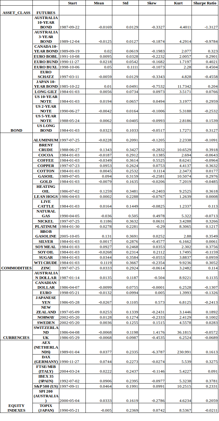
Dataset
For this study, I will be using Futures dataset across 4 asset classes: Indices, Bonds, Currencies, Commodities provided by Quantopian up till 2016.
The continuous dataset is presumably stitched through a backward, forward or proportional adjusted methodology (not explicitly mentioned in Quantopian’s github repository).
Below is the descriptive statistics on 50 instruments used in this study.
Time Series Momentum (TSMOM) methodology
In the AQR papers, the authors experimented with fixed lookback periods of 1 year which determines the trading signal for the next month ie if the price of an asset increase over 1 year period, the trading signal for next month would be Long.
The reverse holds when the price of an asset decreased. Position of each asset is based on lookback exponential standard deviation of daily returns with an annualized volatility of 40%.
The following is the explanation by the authors,

Capital is distributed amongst instruments with available data. For example, if there are only X instruments before 1987, the portfolio returns will be the average of returns from X instruments.
Continuous Forecasts (CF) methodology
In conventional technical analysis, trade entries and exits are usually binary in nature, and current position size is dependent on entry and exit conditions defined t periods ago.
Current position size ~ Entry, exit conditions (dependent on current state) defined t periods ago
But in the financial world, asset returns outcome are continuous in nature with a distribution. Hence it would be optimal for current position size to be directly proportionate to Expected Returns conditional on the current forecast, risk capital allocation, current volatility of instrument, overall portfolio volatility, correlation matrix, cost of rebalancing.
This resonates with the Bayesian school of thought in which probability of hypothesis should be updated as more evidence becomes available.
Current position size ~ E(Returns | current forecast, risk capital, the current volatility of the instrument, overall portfolio volatility, correlation matrix, cost of rebalancing)
The advantage of continuous forecasts approach is that you only need to compare optimal position size given current conditions against current positions. If it diverges by x%, then you rebalance.
The risk management layer and position sizing are inherently built into the framework. And it is not dependent on the state of the current position. This is different from a binary trading system which is state-dependent.
Computation of raw continuous forecasts
For the purpose of my study, I will be considering 2 commonly used technical indicators,
- Exponential moving averages
- Donchian channels
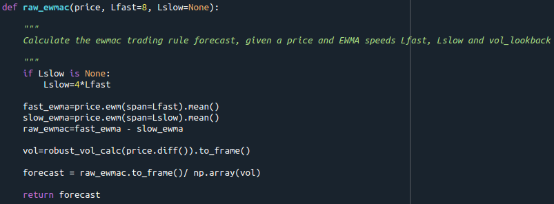
1.1 Exponential moving averages
1) Selection of pairs of fast-moving averages and slow-moving averages to reflect different time-frames: 8-32, 16-64, 32-128, 64-254
2) Raw forecast: First, I take the difference between pair of moving averages
3) Risk-adjusted forecast: Next, I divide the raw forecast by instrument-risk (volatility of instrument in price unit) to get a risk-adjusted forecast.
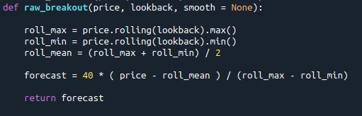
1.2 Donchian Channels
1) Selection of lookbacks to reflect different time-frames: 40, 80, 160, 320
- Forecast: Derived by taking the difference between current price with the middle price (half of max and min over N lookback) divided by difference max and minimum price over N lookback. The formula is as follows, where the 40 multiplier is applied to scale forecasts up to a range of (-20, 20)
\(Forecast\) = \(40\) * \(P_t\) – \((R_{middleN})\) / \((R_{maxN})\) – \((R_{minN})\)
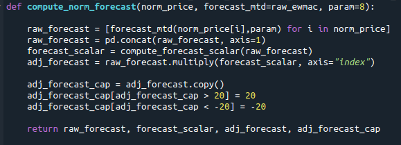
1.3 Forecast scalar
(a) Rescaling forecasts to an average value of 10 for consistency across instruments and time
1) Absolute median forecasts across instruments within a forecast type (eg. 8-32 exponential moving average forecast) is extracted for each day.
2) Next, an expanding window is used to compute the average value of median forecasts in point
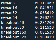
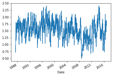
3) Then, I compute the forecast scalar by dividing the average value in point 2 with 10 i.e. we scale the forecast to an average absolute value of 10. 10 represents the average forecast strength for each instrument. In the graphs below, you will notice that forecast scalar plateaus to a level as time progresses (i.e. because of averaging effect over larger data points).
(b) Forecast scalar i.e. multiplier with raw forecasts to scale average forecasts to avg absolute value of 10
EWMAC forecast scalar

Breakout forecast scalar

4) Lastly, the forecast scalar is mapped against the instruments’ individual forecasts time series. Adjusted forecasts are capped between a range of [-20, 20]. This is to avoid overly optimistic or pessimistic forecasts resulting in the outsize position of any particular instrument in the portfolio.

1.4 Combining adjusted forecasts into a weighted forecast for each instrument
From the previous section 1.3(a), I would obtain adjusted forecasts for each instrument. The next step is to combine the forecasts via weights. In this study, I will be using 2 weighting schemes,
1) Equal weight
In the first weighting scheme, I assign equal weights to the rules. In my study, I have 8 different forecasts, 4 for exponential moving averages and 4 for Donchian Channels. 12.5% weight is allocated to each of these forecasts.
2) Weighting through block bootstrapping
In the next weighting scheme, I performed the following steps,
i. Within the in-sample period, I extract 25 blocks of continuous daily periods. Each period accounts for 25% of available days.
ii. For each instrument, I compute the returns stream, \(AR_{it}\) associated with each forecast. First, similar to TSMOM, I find the leverage, \(L_{it}\) required to bring up the realized volatility, \(Vol_{it-1}\) to a reference level of 40%. Next, I scale the leverage up/down according to the strength of the forecasts.\(AR_{it}\) = \(40%\) / \(Vol_{it-1}\) * \(F_{it}\) * \(R_{it}\) = \(L_{it}\) * \(F_{it}\) * \(R_{it}\)
iii. Commission costs of 0.1% is also imposed per trade to penalize frequent rebalancing. Rebalancing only occurs when current forecasts differ from last forecasts by X points (In optimization, found to be 6 points at the overall level).
iv. With the derived returns stream, I proceed to find optimal weights, \(W_{rbi}\) amongst rules, r for the highest Sharpe associated for each bootstrapped block, b per instrument, i.v. Lastly, I pooled the weights together and find the average optimal weights across instruments for an in-sample period,
\(W_r\) = \(Average_{bi}\) \((W_{rbi})\)
Note: Applying optimized weights for each instrument is avoided because of a relatively small number of bootstrapped blocks. And based on Robert Carver’s advice, instruments are more likely to be similar than different in their momentum characteristic. That being said, in my next iteration, I could test this hypothesis.
Scaling up or down at portfolio level according to maximum overall portfolio risk allowed
With diversification across the instruments and forecasts, the realized volatility of the portfolio would be significantly lower than the reference annualized volatility of 40% per instrument. In AQR’s study, the annualized volatility averaged around 12%.
For the purpose of this study, I will use a maximum realized volatility cap at 15%. The steps are as follows:
i. Assume forecasts, \(F_{t-1}\) are at both extreme of -20 and +20 depending on the polarity of the forecasts. And find the maximum realized volatility, \(Mv_{t-1}\)
ii. Next, find the leverage adjustment factor, At at the portfolio level,
\(A_t\) = \(Maximum realized volatility cap of 15%\) / \(Mv_{t-1}\)
Note: During the 2008-2009 crisis, adjustment factor to portfolio dived to 0.50, suggesting that correlation across instruments could have increased.
iii. Last but not the least, I will map the leverage adjustment factor, At to the leverage factor in section 1.4,2,ii. The final leverage, \(FL_{it}\) for the instrument will be as follows:\(FL_{it}\) = \(A_t\) * \(L_{it}\)
iv. In terms of position sizing, let’s say if the instrument is assigned a risk capital of $20,000.
The notional capital, \(NC_{it}\) to be deployed for this instrument would be\(NC_{it}\) = \(FL_{it}\) * $20,000
Note: An alternative is to consider the correlation matrix between instruments and find the adjustment factor.
Evaluation of strategies
I tested the following strategies on in-sample (before 2010-06-07) and out-of-sample periods (after 2010-06-06). Below are the different configurations,
i. TSMOM excluding costs in sample: AQR TSMOM strategy is tested on in-sample period excluding costs.
ii. TSMOM including costs in sample: AQR TSMOM strategy is tested on in-sample period including costs.
iii. Pre-optimize in sample: Equal weights are allocated to different forecasts. And the strategy is tested on the in-sample period.
iv. Optimize in sample: Optimized weights based on block bootstrapping are allocated to different forecasts. And the strategy is tested in-sample period.
v. Pre-optimize out of sample: Equal weights are allocated to different forecasts. And the strategy is tested on ‘out of the sample’ period.
vi. Optimize out of sample: Optimized weights based on block bootstrapping are allocated to different forecasts. And the strategy is tested on of sample period.
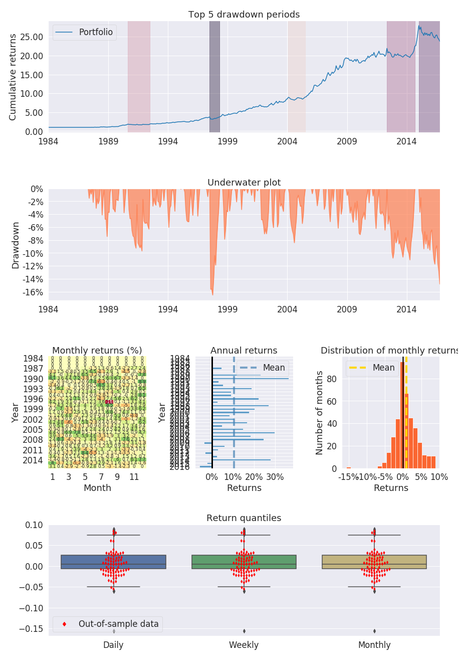
Summary statistics on monthly return
Performance during the in-sample period
Across the board, during the in-sample period, I notice that both types of strategies perform well with Sharpe of > 1, high Calmar ratio, reasonable drawdowns for both TSMOM and continuous forecasts methodology.
Surprisingly, TSMOM 1 year lookback methodology performs better than the continuous forecasts despite the diversification of signals and risk management at the portfolio level.
Performance during out of sample period
During the out-of sample period, risk adjusted returns, sharpe ratio dropped off signficantly with peformance dropping to below 0.7 for both strategies. TSMOM strategy still performs better than continuous forecasts.
According to David Harding, founder of Winton Group and pioneer of quantitative trend following mentioned in an article that one reason for the deterioration in returns could be the overcrowdedness and commoditization of the strategy.
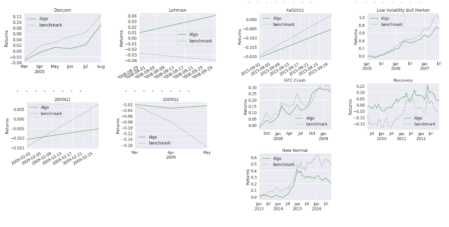
Equity curves of both methodologies

Factor analysis against Fama French 3 factors, Momentum factor, Bonds and Commodity returns
TSMOM in sample data
Factor analysis showed that only Bond and Market(Equity) factors are significant. And TSMOM exhibits a negative beta for Market (Equity) factor and huge beta for the Bond factor. This seems to bode well for a crisis-alpha based strategy as Equities tend to dive during a crisis.

Bootstrap optimized in sample
Similar to TSMOM, the strategy exhibits a negative beta for Market (Equity) factor. This also bodes well for a crisis-alpha based strategy as Equities tend to dive during a crisis.

TSMOM out of sample
Results mirrors in sample data.

Boostrap optimized out of sample
Results do not mirror in sample data. A negative market beta relationship is not present in out of sample data.
Moreover, it exhibits a positive significant relationship with Bonds and negative significant relationship with commodity.

Conclusion
Despite the deterioration in the performance of trend following strategies, it still has a place in an investor’s portfolio. According to Kathryn Kaminski, "trend following exhibits a crisis alpha characteristic".
Future developments for the strategy
In the next iteration, I am keen to explore the feasibility of the strategy beyond 2016 data
At the moment, the data used in this study is stitched together by Quantopian (extracted from Bloomberg). In the next iteration, I am keen to stitch the contracts together either through the forward or backward adjustment method.
With the individual contracts, I am also able to incorporate carry term structure (contango or backwardation) signal into the continuous forecasting system
The block bootstrapped optimization may not have worked well because I only extracted 25 continuous periods from the dataset. Ideally, I would prefer to extract significantly more blocks of data (~1000).
But, I am constrained by computing power. In the next iteration, I would explore using cloud platforms (e.g. Google Collaboratory or AWS) for bootstrap optimization
In the next iteration with more computing power, I would perform a bootstrap optimization and walk-forward analysis. That is to say, I derive optimize weights from t-x to t and test the results on t+1. This will be repeated in each time step with an expanding window.
Disclaimer: The author has no position in this study’s strategy but has keen interests in developing and investing in a viable trend following strategy across asset classes.
References
- Hurst, Brian, Yao Hua Ooi, and Lasse Heje Pedersen. "A century of evidence on trend-following investing." The Journal of Portfolio Management 44, no. 1 (2017): 15-29.
- Moskowitz, Tobias J., Yao Hua Ooi, and Lasse Heje Pedersen. "Time series momentum." Journal of financial economics 104, no. 2 (2012): 228-250.
- Carver, Robert. Systematic Trading: A unique new method for designing trading and investing systems. Harriman House Limited, 2015
- Carver, Robert.Leveraged Trading. Harriman House Limited, 2019.
If you want to learn various aspects of Algorithmic trading then check out the Executive Programme in Algorithmic Trading (EPAT). The course covers various training modules and equips you with the required skill sets to build a promising career in algorithmic trading.
This strategy by Jirong Huang can be seen on his Github page.
Disclaimer: The information in this project is true and complete to the best of our Student’s knowledge. All recommendations are made without guarantee on the part of the student or QuantInsti®. The student and QuantInsti® disclaim any liability in connection with the use of this information. All content provided in this project is for informational purposes only and we do not guarantee that by using the guidance you will derive a certain profit.