Beyond the Straight Line: Advanced Linear Regression Models for Financial Data

By: Aacashi Nawyndder, Vivek Krishnamoorthy and Udisha Alok

Ever feel like financial markets are just unpredictable noise? What if you could find hidden patterns? That's where a cool tool called regression comes in! Think of it like a detective for data, helping us spot relationships between different things.

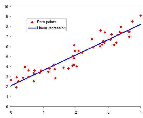
The simplest starting point is linear regression – basically, drawing the best straight line through data points to see how things connect. (We assume you've got a handle on the basics, maybe from our intro blog linked in the prerequisites!).

But what happens when a straight line isn't enough, or the data gets messy? In Part 1 of this two-part series, we'll upgrade your toolkit! We're moving beyond simple straight lines to tackle common headaches in financial modeling. We'll explore how to:

1. Model non-linear trends using Polynomial Regression.
2. Deal with correlated predictors (multicollinearity) using Ridge Regression.
3. Automatically select the most important features from a noisy dataset using Lasso Regression.
4. Get the best of both worlds with Elastic Net Regression.
5. Efficiently find key predictors in high-dimensional data with Least Angle Regression (LARS).

Get ready to add some serious power and finesse to your linear modeling skills!

Prerequisites

Hey there! Before diving in, getting familiar with a few key concepts is a good ideawe dive in, it’s a good idea to get familiar with a few key concepts. You can still follow along without them, but having these basics down will make everything click much easier. Here’s what you should check out:

1. Statistics and Probability
Know the basics—mean, variance, correlation, probability distributions. New to this? Probability Trading is a solid starting point.

2. Linear Algebra Basics
Matrices and vectors come in handy, especially for advanced stuff like Principal Component Regression.

3. Regression Fundamentals
Understand how linear regression works and the assumptions behind it. Linear Regression in Finance breaks it down nicely.

4. Financial Market Knowledge
Brush up on terms like stock returns, volatility, and market sentiment. Statistics for Financial Markets is a great refresher.

Once you've got these covered, you're ready to explore how regression can unlock insights in the world of finance. Let’s jump in!

Acknowledgements

This blog post draws heavily from the information and insights presented in the following texts:

1. Gujarati, D. N. (2011). Econometrics by example. Basingstoke, UK: Palgrave Macmillan.
2. Fabozzi, F. J., Focardi, S. M., Rachev, S. T., & Arshanapalli, B. G. (2014). The basics of financial econometrics: Tools, concepts, and asset management applications. Hoboken, NJ: Wiley.
3. Diebold, F. X. (2019). Econometric data science: A predictive modeling approach. University of Pennsylvania. Retrieved from http://www.ssc.upenn.edu/~fdiebold/Textbooks.html
4. James, G., Witten, D., Hastie, T., & Tibshirani, R. (2013). An introduction to statistical learning: With applications in R. New York, NY: Springer.

Table of contents:

• What Exactly is Regression Analysis?
• So, Why Do We Call These 'Linear' Models?
• Building the Basics
• Advanced Models

What Exactly is Regression Analysis?

At its core, regression analysis models the relationship between a dependent variable (the outcome we want to predict) and one or more independent variables (predictors).

Think of it as figuring out the connection between different things – for instance, how does a company's revenue (the outcome) relate to how much they spend on advertising (the predictor)? Understanding these links helps you make educated guesses about future outcomes based on what you know.

When that relationship looks like a straight line on a graph, we call it linear regression—nice and simple, isn't it?

Before we dive deeper, let's quickly recap what linear regression is.

So, Why Do We Call These 'Linear' Models?

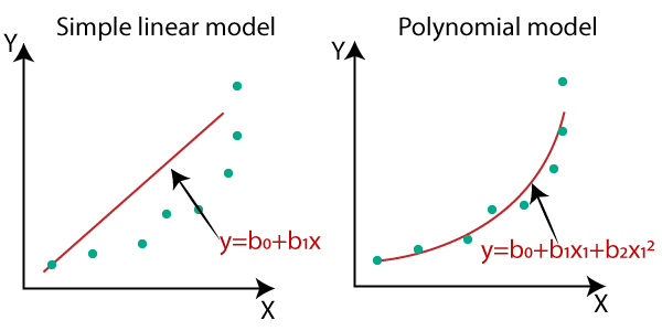
Great question! You might look at something like Polynomial Regression, which models curves, and think, 'Wait, that doesn't look like a straight line!' And you'd be right, visually.

But here's the key: in the world of regression, when we say 'linear,' we're actually talking about the coefficients – those 'beta' values (β) we estimate. A model is considered linear if the equation used to predict the outcome is a simple sum (or linear combination) of these coefficients multiplied by their respective predictor terms. Even if we transform a predictor (like squaring it for a polynomial term), the way the coefficient affects the outcome is still direct and additive.

All the models in this post—polynomial, Ridge, Lasso, Elastic Net, and LARS—follow this rule even though they tackle complex data challenges far beyond a simple straight line.

Building the Basics

From Simple to  Multiple Regression

In our previous blogs, we’ve discussed linear regression, its use in finance, its application to financial data, and its assumptions and limitations. So, we'll do a quick recap here before moving on to the new material. Feel free to skip this part if you're already comfortable with it.

Simple linear regression

Simple linear regression studies the relationship between two continuous variables- an independent variable and a dependent variable.

Source

The equation for this looks like:

$$ y_i = \beta_0 + \beta_1 X_i + \epsilon_i \qquad \text{-(1)} $$

Where:

• \(\beta_0\) is the intercept
• \(\beta_1\) is the slope
• \(\epsilon_i\) is the error term

In this equation, ‘y’ is the dependent variable, and ‘x’ is the independent variable.
The error term captures all the other factors that influence the dependent variable other than the independent variable.

Multiple linear regression

Now, what happens when more than one independent variable influences a dependent variable?  That's where multiple linear regression comes in.

Here's the equation with three independent variables:

$$ y_i = \beta_0 + \beta_1 X_{i1} + \beta_2 X_{i2} + \beta_3 X_{i3} + \epsilon_i \qquad \text{-(2)} $$

Where:

• \(\beta_0, \beta_1, \beta_2, \beta_3\) are the model parameters
• \(\epsilon_i\) is the error term

This extension allows modeling more complex relationships in finance, such as predicting stock returns based on economic indicators. You can read more about them here.

Advanced Models

Polynomial Regression: Modeling Non-Linear Trends in Financial Markets

Linear regression works well to model linear relationships between the dependent and independent variables. But what if the relationship is non-linear?

In such cases, we can add polynomial terms to the linear regression equation to get a better fit for the data. This is called polynomial regression.

Source

So, polynomial regression uses a polynomial equation to model the relationship between the independent and dependent variables.

The equation for a kth order polynomial goes like:

$$ y_i = \beta_0 + \beta_1 X_{i} + \beta_2 X_{i2} + \beta_3 X_{i3} + \beta_4 X_{i4} + \ldots + \beta_k X_{ik} + \epsilon_i \qquad \ $$

Choosing the right polynomial order is super important, as a higher-degree polynomial could overfit the data. So we try to keep the order of the polynomial model as low as possible.

There are two types of estimation approaches to choosing the order of the model:

• Forward selection procedure:
  This method starts simple, building a model by adding terms one by one in increasing order of the polynomial.
  Stopping condition: The process stops when adding a higher-order term doesn't significantly improve the model's fit, as determined by a t-test of the iteration term.
  
• Backward elimination procedure:
  This method starts with the highest order polynomial and simplifies it by removing terms one by one.
  Stopping condition: The process stops when removing a term significantly worsens the model's fit, as determined by a t-test.

Tip: The first- and second-order polynomial regression models are the most commonly used. Polynomial regression is better for a large number of observations, but it's equally important to note that it is sensitive to the presence of outliers.

The polynomial regression model can be used to predict non-linear patterns like what we find in stock prices. Do you want a stock trading implementation of the model? No problem, my friend! You can read all about it here.

Ridge Regression Explained: When More Predictors Can Be a Good Thing

Remember how we talked about linear regression, assuming no multicollinearity in the data? In real life though, many factors can move together. When multicollinearity exists, it can cause wild swings in the coefficients of your regression model, making it unstable and hard to trust.

Ridge regression is your friend here!
It helps reduce the standard error and prevent overfitting, stabilizing the model by adding a small "penalty" based on the size of the coefficients (Kumar, 2019).

This penalty (called L2 regularization) discourages the coefficients from becoming too large, effectively "shrinking" them towards zero. Think of it like gently nudging down the influence of each predictor, especially the correlated ones, so the model doesn't overreact to small changes in the data.
Optimal penalty strength (lambda, λ) selection is important and often involves methods like cross-validation.

Caution:  While the OLS estimator is scale-invariant, the ridge regression is not. So, you need to scale the variables before applying ridge regression.

Ridge regression decreases the model complexity but doesn’t reduce the number of variables (as it can shrink the coefficients close to zero but doesn’t make them exactly zero).
So, it cannot be used for feature selection.

Let’s see an intuitive example for better understanding:

Imagine you're trying to build a model to predict the daily returns of a stock. You decide to use a whole bunch of technical indicators as your predictors – things like different moving averages, RSI, MACD, Bollinger Bands, and many more. The problem is that many of these indicators are often correlated with each other (e.g., different moving averages tend to move together).

If you used standard linear regression, these correlations could lead to unstable and unreliable coefficient estimates. But thankfully, you recall reading that QuantInsti blog on Ridge Regression – what a relief! It uses every indicator but dials back their individual influence (coefficients) towards zero. This prevents the correlations from causing wild results, leading to a more stable model that considers everything fairly.

Ridge Regression is used in various fields, one such example being credit scoring. Here, you could have many financial indicators (like income, debt levels, and credit history) that are often correlated. Ridge Regression ensures that all these relevant factors contribute to predicting credit risk without the model becoming overly sensitive to minor fluctuations in any single indicator, thus improving the reliability of the credit score.
Getting excited about what this model can do? We are too! That's precisely why we've prepared this blog post for you.

Lasso regression: Feature Selection in Regression

Now, what happens if you have tons of potential predictors, and you suspect many aren't actually very useful? Lasso (Least Absolute Shrinkage and Selection Operator) regression can help. Like Ridge, it adds a penalty to prevent overfitting, but it uses a different type (called L1 regularization) based on the absolute value of the coefficients. (While Ridge Regression uses the square of the coefficients.)

This seemingly small difference in the penalty term has a significant impact. As the Lasso algorithm tries to minimize the overall cost (including this L1 penalty), it has a tendency to shrink the coefficients of less important predictors all the way to absolute zero.

So, it can be used for feature selection, effectively identifying and removing irrelevant variables from the model.

Note: Feature selection in Lasso regression is data-dependent (Fonti, 2017).

Below is a really useful example of how Lasso regression shines!

Imagine you're trying to predict how a stock will perform each week. You've got tons of potential clues – interest rates, inflation, unemployment, how confident consumers are, oil and gold prices, you name it. The thing is, you probably only need to pay close attention to a few of these.

Because many indicators move together, standard linear regression struggles, potentially giving unreliable results. That's where Lasso regression steps in as a smart way to cut through the noise. While it considers all the indicators you feed it, its unique L1 penalty automatically shrinks the coefficients (influence) of less useful ones all the way to zero, essentially dropping them from the model. This leaves you with a simpler model showing just the key factors influencing the stock's performance, instead of an overwhelming list.

This kind of smart feature selection makes Lasso really handy in finance, especially for things like predicting stock prices. It can automatically pick out the most influential economic indicators from a whole bunch of possibilities. This helps build simpler, easier-to-understand models that focus on what really moves the market.

Want to dive deeper? Check out this paper on using Lasso for stock market analysis.

Elastic net regression: Combining Feature Selection and Regularization

So, we've learned about Ridge and Lasso regression. Ridge is great at shrinking coefficients and handling situations with correlated predictors, but it doesn't zero out coefficients entirely (keeping all features) while Lasso is excellent for feature selection, but may struggle a bit when predictors are highly correlated (sometimes just picking one from a group somewhat randomly).

What if you want the best of both? Well, that's where Elastic Net regression comes in – an innovative hybrid, combining both Ridge and Lasso Regression.

Instead of choosing one or the other, it uses both the L1 penalty (from Lasso) and the L2 penalty (from Ridge) together in its calculations.

Source

How does it work?

Elastic Net adds a penalty term to the standard linear regression cost function that mixes the Ridge and Lasso penalties. You can even control the "mix" – deciding how much emphasis to put on the Ridge part versus the Lasso part. This allows it to:

1. Perform feature selection like Lasso regression.
2. Provide regularization to prevent overfitting.
3. Handle Correlated Predictors: Like Ridge, it can deal well with groups of predictors that are related to each other. If there's a group of useful, correlated predictors, Elastic Net tends to keep or discard them together, which is often more stable and interpretable than Lasso's tendency to pick just one.

You can read this blog to learn more about ridge, lasso and elastic net regressions, along with their implementation in Python.

Here's an example to make it clearer:

Let's go back to predicting next month's stock return using many data points (past performance, market trends, economic rates, competitor prices, etc.). Some predictors might be useless noise, and others might be related (like different interest rates or competitor stocks). Elastic Net can simplify the model by zeroing out unhelpful predictors (feature selection) and handle the groups of related predictors (like interest rates) together, leading to a robust forecast.

Least angle regression: An Efficient Path to Feature Selection

Now, imagine you're trying to build a linear regression model, but you have a lot of potential predictor variables – maybe even more variables than data points!

This is a common issue in fields like genetics or finance. How do you efficiently figure out which variables are most important?

Least Angle Regression (LARS) offers an interesting and often computationally efficient way to do this. Think of it as a smart, automated process for adding predictors to your model one by one, or sometimes in small groups. It's a bit like forward stepwise regression, but with a unique twist.

How does LARS work?

LARS builds the model piece by piece focusing on the correlation between the predictors and the part of the dependent variable (the outcome) that the model hasn't explained yet (the "residual"). Here’s the gist of the process:

1. Start Simple: Begin with all predictor coefficients set to zero. The initial "residual" is just the response variable itself.
2. Find the Best Friend: Identify the predictor variable with the highest correlation with the current residual.
3. Give it Influence: Start increasing the importance (coefficient) of this "best friend" predictor. As its importance grows, the model starts explaining things, and the leftover "residual" shrinks. Keep doing this just until another predictor perfectly matches the first one in how strongly it's linked to the current residual.
4. The "Least Angle" Move: Now you have two predictors tied for being most correlated with the residual. LARS cleverly increases the importance of both these predictors together. It moves in a specific direction (called the "least angle" or "equiangular" direction) such that both predictors maintain their equal correlation with the shrinking residual.

Geometric representation of LARS: Source

1. Keep Going: Continue this process. As you go, a third (or fourth, etc.) predictor might eventually catch up and tie the others in its connection to the residual. When that happens, it joins the "active set" and LARS adjusts its direction again to keep all three (or more) active predictors equally correlated with the residual.
2. Full Path: This continues until all predictors you're interested in are included in the model.

LARS and Lasso:

Interestingly, LARS is closely related to Lasso regression. A slightly modified version of the LARS algorithm is actually a very efficient way to compute the entire sequence of solutions for Lasso regression across all possible penalty strengths (lambda values). So, while LARS is its own algorithm, it provides insight into how variables enter a model and gives us a powerful tool for exploring Lasso solutions.

But, why use LARS?

• It's particularly efficient when you have high-dimensional data (many, many features).
• It provides a clear path showing the order in which variables enter the model and how their coefficients evolve.

Caution: Like other forward selection methods, LARS can be sensitive to noise.

Use case: LARS can be used to identify Key Factors Driving Hedge Fund Returns:

Imagine you're analyzing a hedge fund's performance. You suspect that various market factors drive its returns, but there are dozens, maybe hundreds, you could consider: exposure to small-cap stocks, value stocks, momentum stocks, different industry sectors, currency fluctuations, etc. You have way more potential factors (predictors) than monthly return data points.

Running standard regression is difficult here. LARS handles this "too many factors" scenario effectively.

Its real advantage here is showing you the order in which different market factors become essential for explaining the fund's returns, and exactly how their influence builds up.

This gives you a clear view of the primary drivers behind the fund's performance. And helps build a simplified model highlighting the key systematic drivers of the fund's performance, navigating the complexity of numerous potential factors efficiently.

Summary

Conclusion

Phew! We've journeyed far beyond basic straight lines!

You've now seen how Polynomial Regression can capture market curves, how Ridge Regression stabilizes models when predictors move together, and how Lasso, Elastic Net, and LARS act like smart filters, helping you select the most crucial factors driving financial outcomes.

These techniques are essential for building more robust and reliable models from potentially complex and high-dimensional financial data.

But the world of regression doesn't stop here! We've focused on refining and extending linear-based approaches.

What happens when the problem itself is different? What if you want to predict a "yes/no" outcome, focus on predicting extreme risks rather than just the average, or model incredibly complex, non-linear patterns?

That's precisely what we'll tackle in Part 2! Join us next time as we explore a different side of regression, diving into techniques like Logistic Regression, Quantile Regression, Decision Trees, Random Forests, and Support Vector Regression. Get ready to expand your predictive modeling horizons even further!

Getting good at this stuff really comes down to rolling up your sleeves and practicing! Try playing around with these models using Python or R and some real financial data – you'll find plenty of tutorials and projects out there to get you started.

For a complete, holistic view of regression and its power in trading, you might want to check out this Quantra course.

And if you're thinking about getting serious with algorithmic trading, checking out something like QuantInsti’s EPAT program could be a great next step to really boost your skills for a career in the field.

Understanding regression analysis is a must-have skill for anyone aiming to succeed in financial modeling or trading strategy development.

So, keep practicing—and soon you'll be making smart, data-driven decisions like a pro!

With the right training and guidance from industry experts, it can be possible for you to learn it as well as Statistics & Econometrics, Financial Computing & Technology, and Algorithmic & Quantitative Trading. These and various aspects of Algorithmic trading are covered in this algo trading course. EPAT equips you with the required skill sets to build a promising career in algorithmic trading. Be sure to check it out.

References

1. Fonti, V. (2017). Feature selection using LASSO. Research Paper in Business Analytics. Retrieved from https://vu-business-analytics.github.io/internship-office/papers/paper-fonti.pdf
2. Kumar, D. (2019). Ridge regression and Lasso estimators for data analysis. Missouri State University Theses, 8–10. Retrieved from https://bearworks.missouristate.edu/cgi/viewcontent.cgi?article=4406&context=theses
3. Efron, B., Hastie, T., Johnstone, I., & Tibshirani, R. (2003, January 9). Least Angle Regression. Statistics Department, Stanford University.
   https://hastie.su.domains/Papers/LARS/LeastAngle_2002.pdf
4. Taboga, Marco (2021). "Ridge regression", Lectures on probability theory and mathematical statistics. Kindle Direct Publishing. Online appendix. https://www.statlect.com/fundamentals-of-statistics/ridge-regression

Disclaimer: All investments and trading in the stock market involve risk. Any decision to place trades in the financial markets, including trading in stock or options or other financial instruments, is a personal decision that should only be made after thorough research, including a personal risk and financial assessment and the engagement of professional assistance to the extent you believe necessary. The trading strategies or related information mentioned in this article is for informational purposes only.