This article was originally posted on Quants Portal.
The Monte Carlo, filled with a lot of mystery is defined by Anderson et al (1999) as the art of approximating an expectation by the sample mean of a function of simulated variables. Used as a code word between Stan Ulam and John von Neumann for the stochastic simulations they applied to build better atomic bombs (Anderson, 1999), the term Monte Carlo evolved into a method used in a variety discipline including physic, finance, mechanics and even in areas such as town planning and demographic studies.
Monte Carlo methods are very different from deterministic methods (McLeish, 2004). In the case of a deterministic model the value of the dependent variable, given the explanatory variables, can only be unique value as given by a mathematical formula. This type of model contains no random components (Rotelli, 2015). In contrast, Monte Carlo does not solve an explicit equation but rather obtains answers by simulating individual particles and recording some aspects (tallies) of their average behaviour (Briesmeister, 2000). Given the broad applications and matters involving Monte Carlo Methods, we will split this article into three parts to allow for a clear understanding.
First I give a brief history behind Monte Carlo methods then highlight some of its uses by taking an example in physics and showing its necessity in finance, then conclude with what is known as importance sampling for those statistically driven.
In later writings, we will delve more on the technical side of things giving strict definitions of significant concepts then progress to discuss Markov Chain Monte Carlo (MCMC) as they form a great role in recent MC computations. In my last offering, I will combine all these aspects to form a solid and holistic understanding of the “Black-Box” called Monte Carlo Methodologies with the spotlight on the Metropolis-Hasting algorithm and explore future possibilities within Ulan and von Neumann’s creation.
Monte Carlo’s History
Just as an apple landed on Newton’s head ignited a new stream of science, Stan Ulan had to be sick for him to discover what developed to be an answer for a vast number of scientific problems. Though Ulam and von Neumann formalized and coined the term Monte Carlo, earlier evidence of the approximation method exists. Most notable is the Buffon’s needle experiment. This experiment is as follows:
“A needle of length L is thrown in a random fashion onto a smooth table ruled with parallel lines separated by a distance of 2L. An observer records whether or not the needle intersects a ruled line. From the experiment, it is deduced that as the sample increases the probability of the needle crossing the line tends to 1/pi.”(Schuster, 1974).
Ulan in 1964 while in his sick bed wondered if a Canfield Solitaire laid out with 52 cards will successfully be observed. After some thoughts and using pure mathematical methods he played the game 100 times and noted all the successful plays and the proportion of the wins reflected the odds of getting a winning hand. He obtained his results and soon enough he postulated problems on most mathematical physics and on differential equations that would benefit from this practical way of calculation. Later that year he conferred the idea to a John von Neumann (Eckhardt, 1987)with whom they started more complex computational problems and later working on nuclear weapons.
The name Monte Carlo is also inspired by the game of roulette played in Monaco which was a game involving simple random number generation. Another somewhat comical motive was because Ulan’s uncle enjoyed visiting the Monte Carlo to play this roulette as such it was in his honour.
Applications of Monte Carlo
As mentioned above Monte Carlo methods can be applied in many fields of studies. The very first applications were done by the inventors where they used MC methods in solving problems of neutron diffusion and multiplication problems in fission devices using Electronic Numeric Integrator and Calculator(ENIAC). This later developed into the MCNP.

Application in Physical Sciences
Monte Carlo N–Particle (MCNP) is a general-purpose, continuous-energy, generalized-geometry, time-dependent, coupled neutron/photon/electron Monte Carlo transport code. It can be used in several transport modes: neutron only, photon only, electron only, combined neutron/photon transport where the photons are produced by neutron interactions, neutron/photon/electron, photon/electron, or electron/photon.
Though the jargon can be confusing, assuming very little knowledge of the Monte Carlo method and no experience with MCNP Judith F. Briesmeister maintains that even novice may grasp the concepts (Briesmeister, 2000), with practice of course.
Application in Finance
The MC approach has proved to be a valuable and flexible computational tool in modern finance. With a focus on asset pricing: basic securities and their underlying state variables are often modelled as continuous-time stochastic processes. It was only a matter of time before Monte Carlo methods were used in the evaluation of security prices represented as expectation (Boyle, Broadie, & Glasserman, 1997). We can clearly see the need for MC methods in pricing derivatives and other financial products due to its flexibility in handling increasingly complex financial instruments. A detailed example of the use of Monte Carlo methods in finance is provided in the third part of this article.
Importance Sampling
Importance sampling is choosing a good distribution from which to simulate random variables (Anderson E. C., 1999). It makes intuitive sense that we must obtain a sample from important regions so as to obtain accurate results. This is done by overweighing important regions within the sample; hence the name importance sampling. Contrary to its name importance sampling is not sampling per se but rather an approximation method. Let us at this point explore importance sampling in an intuitive manner:
Assuming we wish to perform an analysis on a factor but do not have the relevant data to which we can perform the analysis or the data we have does not offer sufficient results. We then generate a random sample which complies with the following properties:
Let g(x) be the original sample distribution (if it exists) and h(x) be the proposed sample distribution.
- h(x) should be close to being proportional to |g(x)|
- it should be easy to simulate values from h(x)
- It should easy to compute the density h(x) for any value x that may be realized.
Adhering to these requirements may be very difficult to require sufficient time investment but proves to be effective in dealing with the two problems mentioned above. I chose to include importance sampling at this stage as it is edifying for later discussions more so with regards to Monte Carlo improvement techniques. We will discover that there is an important relationship between importance sampling and Markov Chains.
We have defined a Monte Carlo as an approximation technique which has vast usage and learned of it’s intriguing and somewhat throbbing history (throbbing because the name’s nature of being associated with bomb constructions). Having developed from using ENIAC by von Neumann to being used by modern computers, MC play a large role in the simulation and manipulation of data/processes which has had tremendous effects in the way we live and how to interact with our world.
In the next part of the article, we go more in-depth and explore other components inherent in the MC and discuss the Metropolis-Hasting Algorithm as a special case of Monte Carlo Markov Chain process.
Markov Chains, Central Limit Theorem and the Metropolis-Hastings
In the previous section of the article, I gave a generic overview of Monte Carlo as well as introduced importance sampling. We now dive deeper by giving strict definitions of some of the widely used and yet misunderstood or rather commonly neglected concepts due to its perceived importance. Thereafter, we explore the Metropolis-Hastings algorithm which forms a foundation of numerous Markov Chain Monte Carlo methods.
Markov Chains Monte Carlo
Markov Chains were invented soon after ordinary Monte Carlo by Los Alamos who used computation to obtain such simulations. The chains are classically obtained from following the variety of algorithms with the Metropolis algorithm being the most embryonic and yet significant as it paved the way for more elaborate algorithms like the Metropolis-Hasting algorithm. Since Monte Carlo integrations draw samples from a required distribution and form sample averages to approximate expectation, the Markov Chains Monte Carlo draw these samples by running cleverly constructed Markov chains for a long time (Gilks, Richardson, & Spiegelhalter)
Let us at this point give strict definitions of some important terms and concepts (Some definitions are extracted from Geyer C.J: Introduction to Markov Chain Monte Carlo):
Definitions
Markov Chain: A sequence X1, X2, X3, … of random elements of some set is a Markov chain if the conditional distribution of Xn+1 given X1, X2, X3, … , only depends on Xn. From this definition, we see that in order to compute the next random variable we only need current information and nothing before where we currently stand thus greatly reducing the time spent on sourcing and calculation time.
Reversibility: A transition probability distribution is reversible with respect to the initial distribution if, of a Markov Chain X1, X2, X3, … the distribution of pairs are exchangeable. Reversibility eases the applications of the central limit Theorem (CLT) as the conditions of the CLT are much simpler when this property holds.
Stationarity: A stochastic process (xt : t in an element of the parameter space) is stationary if all Xt have the same mean, variance and autocorrelation
Central Limit Theorem: For a stationary, irreducible, reversible Markov Chain and ![]() and μ as well as variance σ² with σ² finite then
and μ as well as variance σ² with σ² finite then ![]() where
where ![]() is the sample estimate. We can further explain it in a general manner as follows: for any sequence of random variables X1, X2, X3, … with X1, X2, X3, … independently identically distributed, the joint distribution function as n tends to infinity is given by a Normal (0, σ²) distribution. It is worth noting that various forms of the CLT exists all with their specific requirements
is the sample estimate. We can further explain it in a general manner as follows: for any sequence of random variables X1, X2, X3, … with X1, X2, X3, … independently identically distributed, the joint distribution function as n tends to infinity is given by a Normal (0, σ²) distribution. It is worth noting that various forms of the CLT exists all with their specific requirements
Monte Carlo Estimates and Central Limit Theorem
In order to use the CLT to estimate the Monte Carlo error (not discussed here but equally significant), we need a consistent estimate of the variance or at least a variance estimate whose asymptotic distribution is known (Geyer, 1992). Many methods of variance estimation have been proposed, most coming from time series literature and are applicable to arbitrary stationary stochastic processes, not just to Markov chains (Geyer, 1992). We now look at one such method for standard time series.
Non-overlapping Batch Means
Under the Non-overlapping Batch Means (batch: being a subsequence of conservative iterations of the Markov chain with n terms X1, X2,……. XT and assuming a stationary Markov Chain we will have that all the batches of the same length have the same joint distribution (Geyer, 1992). Also, the Central Limit Theorem will apply to each batch.
The batch mean is given by
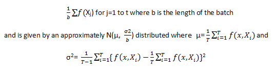
This variance will then be used in the computation of our Central limit theorem.
Metropolis-Hasting Algorithm
The Metropolis-Hastings algorithm is given by the following steps given x(t)
1 Generate ![]()
2 Take 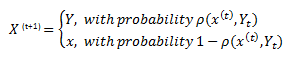
We call p(x, y) the acceptance probability. By performing this process we obtain the so-called Metropolis Hasting Markov Chain X1, X2,……. XT with XT approximately distributed according to (x). (f(x) is what we may consider our ideal sample distribution) for large T. (Kroese, Taimre, & Botev, 2011).
The main aim behind the Metropolis-Hasting is to simulate a Markov chain such that the stationary distribution of this chain coincides with the target distribution.
Though MC method are often more efficient than conventional numeric methods its implementation can be very difficult as well as expensive to compute both in time and analysis. Hastings proposes a generalized method which stems from Metropolis et al (1953). The main features of this sampling method is that
- The computation depends on p(x) only through ratios of the form p(x')/p(x) where x' and x are sample points eliminating the need to factorize p(x) nor determine the normalizing constant
Further literature is available on Metropolis-Hastings but what we highlighted is sufficient at this point. Ideally what we try to do with algorithms like the Metropolis is to come up with a sample that is as close to reality as possible thus ensuring whichever proposed model is tested under as realistic settings as possible.
We have to this point gathered enough theoretical knowledge to structure a strategy that may be employed for investment usage. In our last part of the article, we will make use of all concepts developed uptil now to evaluate their significance.
Financial Applications
Within the Monte Carlo realm, a vast number of applications exist. In this final part, I bring together all the previous work as well as put into practice the theory we have gathered so far.
Applying the Metropolis-Hastings Algorithm
From the previous section, we deduced a way in which we can generate a sample using arbitrary factors which combined produce a fairly accurate representation of reality
For absolute simplicity, we will consider only one variable in which we wish to model, but this process is applicable to combinations of assets or derivatives of those assets with minimal adjustments. Here we make use of Dynamic asset pricing to estimate equilibrium as well as exploit arbitrage opportunities with the theory of mean reversion being the basis of our strategy. I will neglect the actual computation to give an intuitive understanding of the usage of the theory developed here:
- Suppose an asset A has considerable volatility and we desire to capitalize on this observation. The algorithm we have enables us to simulate our own stock movement and match it against A’s movements.
- Assuming a Brownian motion as our q(x) (proposal distribution) we apply the Metropolis-Hastings Algorithm recording all observations.
At this point we have two alternatives of methods we can use for comparison:
Alternative 1: Since we have a defined process we can directly plot this pseudo-trend against the observed trend then make trade decisions based on the price differences. We then structure a program to make buy and sell decisions based on the relation between the two.
- When the generated process is above the assets price this would reflect a buy as we assume the prices will retract to our model (Remember that our model gives a stationary distribution implying that as time goes on prices will converge to this steady state (Johannes & Polson, 2002))
- For the generated process below the assets price, a sell trigger will be executed.
Alternative 2: To further strengthen our decision we may use a regression model based on the generated sample path. By so doing we are capable of even hypothesizing a future trend of asset A’s movement while having an understanding and control of current price fluctuations. Also, the trade decisions applied in the first model may also be applied using the regression model as a benchmark.
This is an overly Simplified model which only gives an idea a possible use. The use of Brownian motion is included as our q based on its properties to model financial movements and the inclusion of noise within its computation (Morters & Peres, 2008). Also although theoretically, we do not place restrictions on q, it is important to note that the choice of the proposal density will generally affect the performance of the algorithm. (Johannes & Polson, 2002, p. 26)
Barrier Options and Importance Sampling
We almost always consider vanilla options when describing and working with options and assume the same applies to exotic types. I will take a slightly different path and consider an exotic option; a barrier option to be exact. The following Example is extracted from the Handbook of Monte Carlo Methods by Kroese D,P Taime T and Botev Z,I:
Consider a Down-and-in call option with a monitored barrier and a payoff at maturity given by
![]()
where 
With ![]() and
and ![]() for k = 1, 2, 3,….,n. The event of a positive payoff in this option can be rare and hence computation of the option price is greatly dependent on rare occurrences. As such estimating a robust probability is imperative and importance sampling may play an enormous role.
for k = 1, 2, 3,….,n. The event of a positive payoff in this option can be rare and hence computation of the option price is greatly dependent on rare occurrences. As such estimating a robust probability is imperative and importance sampling may play an enormous role.
Furthermore: to obtain a good impotence sampling density we use what is known as the Cross-Entropy method. This among other things involve obtaining a pdf of the form
![]()
where ![]() the pdf of a standard normal random vector Ζ. Further enhancements of the proposed pdf may be acquired by using a variation of the Metropolis-Hasting algorithm called the hit-and-run algorithm.
the pdf of a standard normal random vector Ζ. Further enhancements of the proposed pdf may be acquired by using a variation of the Metropolis-Hasting algorithm called the hit-and-run algorithm.
Concluding Note and Summary
Metropolis-Hastings methodology has an immense application which we may not discuss in single blog series, despite its general acceptance only in the 1990s (Hitchocock, 2012). Various adaptations of the Metropolis-Hastings algorithm including the Independence samplers and Random walk sampler further work to provide more relevant predictions. Hastings who saw transition matrices of the Markov chains central to the Metropolis presented his target distributions as an invariant distribution of Π(x) of Markov Chains (Hitchocock, 2012, p. 155), a feature that as mentioned before has reshaped many disciplines.
The whole purpose of all these exercises at the end of the day is to come up with a sample that closely emulates reality but within our control. With this in mind numerous variance reduction techniques which aim to utilize known information about the model to obtain more accurate estimators exists (Kroese & Rubinstein, 2008). We briefly touched on one such technique in part two being the Non-Overlapping Batch means. Other well-known techniques that may provide moderate variance reduction include the use of control and/or arithmetic random variables, stratified sampling (Kroese & Rubinstein, 2008) and the all favourite Importance sampling. (Kroese, Tamimre, & Botev, 2011)
Kroese et al consider Importance sampling one of the most important variance reduction technique (2011, p.362) more so in its ability in finding estimations for rare-event probabilities. As with most topics discussed in this series, only introductory material is given here with vast derivations of the sampling methods are found within academic literature.
For robust results, the inclusion of the Cross-Entropy is beneficial. The intention of the Cross-Entropy method is to obtain density such that the distance between this density and the optimal density (reality) is as small as possible. Weighted Importance sampling is a variation which is most relevant for financial markets as it allocates more weight to factors that have significant input on the process.
Applying all these methods in unison will greatly increase returns and drastically mitigate risk as well as assist in forming resistant investment strategy.
Bibliography
- Anderson, E. (1999). Monte Carlo Method and Importance sampling.
- Boyle, P., Broadie, M., & Glasserman, P. (1997). Monte Carlo Methods for Security Pricing. Journal of Economics and Control, 1267-1321.
- Briesmeister, J. F. (2000). MCNP- A General Monte Carlo N-Particle Transport Code.
- Eckhardt, R. (1987). Stan Ulam, John von Neumann, and the Monte Carlo Method. Obtained from ScienceMadness.org.
- Geyer, C. J. (1992). Practical Markov Chain Monte Carlo. Statistical Science vol 7 No 4, 473-483.
- Gilks, W. R., Richardson, S., & Spiegelhalter, D. J. (n.d.). Introducing Markov Chain Monte Carlo.
- Hitchocock, D. B. (2012). A History of the Metropolis-Hasting Algorithm. The American Statistician, 254-257.
- Johannes, M., & Polson, N. (2002). MCMC Methods for Financial E.
- Kroese, D. P., Tamimre, T., & Botev, Z. I. (2011). Handbook of Monte Carlo Methods. Hoboken New Jersey: John Wiley & Sons Inc.
- Kroese, D. P., & Rubinstein, R. Y. (2008). Simulation and the Monte Carlo Method. New Jersey: John Wiley & Sons, INC.
- Kroese, D., Taimre, T., & Botev, Z. I. (2011). Hand Book of Monte Carlo Methods. New Jersey: John Wiley & Sons.
- Morters, P., & Peres, Y. (2008). Brownian Motion.
- McLeish, D. L. (2004). Monte Carlo Simulation and Finance.
- Rotelli, F. (2015). Stochastic Processes. Pretoria.
- Schuster, E. F. (1974). Buffon’s Needle Experiment. Mathematical Association of America.
- Xu, H., & Zhang, D. (2010). Monte Carlo for Mean-Risk Optimization and Portfolio Selection. Southhampton: University of Southhampton.
Disclaimer: The views, opinions, and information provided within this guest post are those of the author alone and do not represent those of QuantInsti®. The accuracy, completeness, and validity of any statements made or the links shared within this article are not guaranteed. We accept no liability for any errors, omissions or representations. Any liability with regards to infringement of intellectual property rights remains with them.