Machine Learning Classification: Concepts, Models, Algorithms and more

Updated By Chainika Thakar. (Originally written by Kshitij Makwana and Satyapriya Chaudhari)

In the realm of machine learning, classification is a fundamental tool that enables us to categorise data into distinct groups. Understanding its significance and nuances is crucial for making informed decisions based on data patterns.

Let me start by asking a very basic question.
What is Machine Learning?

Machine learning is the process of teaching a computer system certain algorithms that can improve themselves with experience. A very technical definition would be:

"A computer program is said to learn from experience E with respect to some task T and some performance measure P, if its performance on T, as measured by P, improves with experience."
-  Tom Mitchell, 1997

Just like humans, the system will be able to perform simple classification tasks and complex mathematical computations like regression. It involves the building of mathematical models that are used in classification or regression.

To ‘train’ these mathematical models, you need a set of training data. This is the dataset over which the system builds the model. This article will cover all your Machine Learning Classification needs, starting with the very basics.

Coming to machine learning algorithms, the mathematical models are divided into two categories, depending on their training data - supervised and unsupervised learning models.

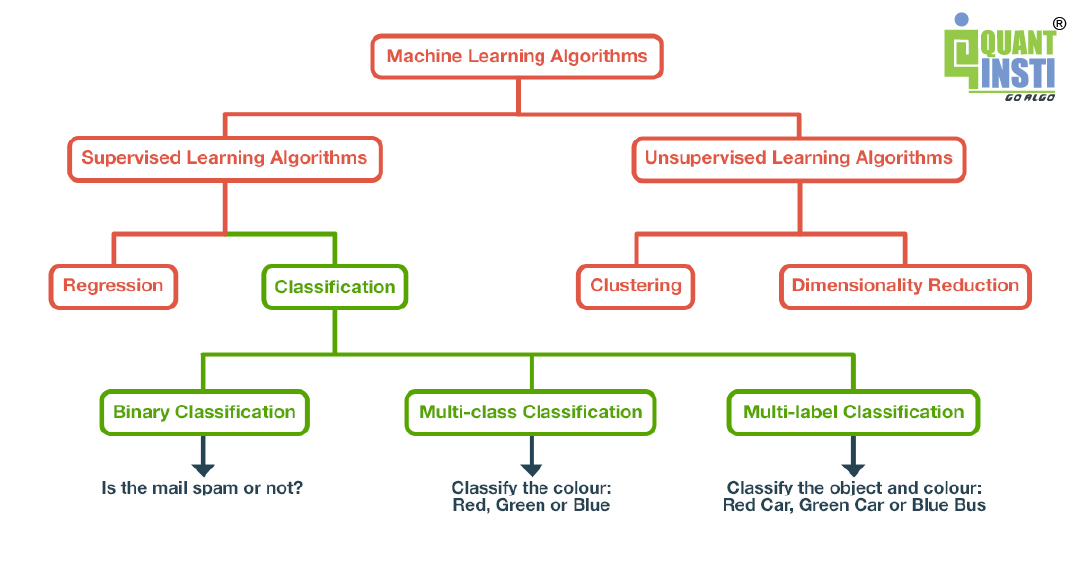
Supervised Learning

When building supervised learning models, the training data used contains the required answers. These required answers are called labels. For example, you show a picture of a dog and also label it as a dog.

So, with enough pictures of a dog, the algorithm will be able to classify an image of a dog correctly. Supervised learning models can also be used to predict continuous numeric values such as the price of the stock of a certain company. These models are known as regression models.

In this case, the labels would be the price of the stock in the past. So the algorithm would follow that trend.

Few popular algorithms include:

• Linear Regression
• Support Vector Classifiers
• Decision Trees
• Random Forests

Unsupervised Learning

In unsupervised learning, as the name suggests, the dataset used for training does not contain the required answers. Instead, the algorithm uses techniques such as clustering and dimensionality reduction to train.

A major application of unsupervised learning is anomaly detection. This uses a clustering algorithm to find out major outliers in a graph. These are used in credit card fraud detection. Explore the 'unsupervised learning course' from Quantra.

Since classification is a part of supervised learning models, let us find out more about the same.

Types of Supervised Models

Supervised models are trained on labelled dataset. It can either be a continuous label or categorical label. Following are the types of supervised models:

• Regression
• Classification

Regression models

Regression is used when one is dealing with continuous values such as the cost of a house when you are given features such as location, the area covered, historic prices etc. Popular regression models are:

• Linear Regression
• Lasso Regression
• Ridge Regression

Classification models

Classification is used for data that is separated into categories with each category represented by a label. The training data must contain the labels and must have sufficient observations of each label so that the accuracy of the model is respectable. Some popular classification models include:

• Support Vector Classifiers
• Decision Trees
• Random Forests Classifiers

There are various evaluation methods to find out the accuracy of these models also. We will discuss these models, the evaluation methods and a technique to improve these models called hyperparameter tuning in greater detail.

Some of the concepts covered in this blog are taken from this Quantra course on Trading with Machine Learning: Classification and SVM. You can take a Free Preview of the course.

Now that you have got a brief idea about Machine Learning and Classification, let us dive further in this journey to master the art of machine learning classification as this blog covers:

• General examples of Machine Learning classification
• Types of classification problems
• Importance of classification in Machine Learning from trading point of view
• What is the difference between SVM and other classification algorithms?
• Preparing Data for Classification
  • Data Collection and Preprocessing
  • Data Exploration and Visualisation
  • Feature Selection and Engineering
• Fundamental Concepts
  • Supervised Learning Overview
  • Training and Testing Data Split
  • Evaluation Metrics for Classification
• Classification Algorithms
  • Linear Models
  • Tree-Based Methods
  • Support Vector Machines
  • Nearest Neighbors
  • Naive Bayes
  • Neural Networks
  • Ensembles
• Challenge: Handling Imbalanced Data
  • Techniques for Imbalanced Datasets
  • Resampling Methods
• Hyperparameter Tuning or Model Optimisation
  • Grid Search
  • Random Search
  • Bayesian Optimisation
• Model Evaluation and Selection
  • Cross-Validation
  • Model Selection Strategies
  • Interpretability and Explainability
• Using SVC in trading
• Resources to learn Machine Learning Classification

General examples of Machine Learning classification

Let us now see some general examples of classification below to learn about this concept properly.

Email Spam Detection

• In this example of email spam detection, the categories can be “Spam” and “Not Spam”.
• If an incoming email contains phrases like "win a prize", "free offer" and "urgent money transfer", your spam filter might classify it as "Spam".
• If an email contains professional language and is from a known contact, it might classify it as "Not Spam".

Disease Diagnosis

• In disease diagnosis, let us assume that two categories are "Pneumonia" and "Common Cold".
• If a patient's medical data includes symptoms like high fever, severe cough, and chest pain, a diagnostic model might classify it as "Pneumonia".
• If the patient's data indicates mild fatigue and occasional headaches, the model might classify it as "Common Cold".

Sentiment Analysis in Social Media

• In this example of sentiment analysis, we can have two categories, namely "Positive" and "Negative".
• If a tweet contains positive phrases like "amazing", "great experience", and "highly recommend", a sentiment analysis model might classify it as "Positive".
• If a tweet includes negative terms such as "terrible", "disappointed" and "waste of money", it might classify it as "Negative".

Types of classification problems

Here are the types of classification problems commonly encountered in machine learning:

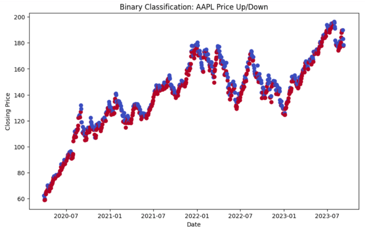
Binary Classification

In this type, the goal is to classify data into one of two classes or categories. For example, spam detection (spam or not spam), disease diagnosis (positive or negative), or customer churn prediction (churn or no churn) are binary classification problems.

Let us take an example. We will take data from APPLE for which the duration will range from 2020-03-30 to 2023-09-10.

Output:

                 Open       High        Low      Close     Volume  \
Date                                                                
2020-03-30  61.295327  62.463835  60.967751  62.290268  167976400   
2020-03-31  62.483378  64.167688  61.603329  62.163136  197002000   
2020-04-01  60.258813  60.801510  58.457162  58.892296  176218400   
2020-04-02  58.752952  59.928792  57.912017  59.875011  165934000   
2020-04-03  59.354319  60.063244  58.418045  59.014523  129880000   

            Price_Up_Down  
Date                       
2020-03-30              0  
2020-03-31              0  
2020-04-01              1  
2020-04-02              0  
2020-04-03              1  

In this binary classification example above, we created a target variable 'Price_Up_Down' to predict whether the stock price will go up (1) or down (0) the next day.

Multi-Class Classification

In multi-class classification, data is divided into more than two distinct classes. Each data point belongs to one and only one class. Examples include classifying emails into multiple categories (e.g., work, personal, social) or recognising different species of plants (e.g., rose, tulip, daisy).

Output:

[*********************100%%**********************]  1 of 1 completed
Accuracy: 0.49
Classification Report:
              precision    recall  f1-score   support

    Decrease       0.47      0.38      0.42        21
    Increase       0.50      0.61      0.55        23
        Stay       0.00      0.00      0.00         1

    accuracy                           0.49        45
   macro avg       0.32      0.33      0.32        45
weighted avg       0.48      0.49      0.48        45

The example above creates a scatter plot where data points are colour-coded based on the price change categories: "Increase", “Decrease” and “Stay”.

The model achieved an accuracy of 0.49, which means it correctly classified approximately 49% of the samples in the test dataset.

The x-axis represents the MACD values, and the y-axis represents the RSI values.

The classification report provides a more detailed evaluation of the model's performance for each class (in our case, "Decrease," "Increase," and "Stay").

Here's what each metric in the report signifies:

• Precision: Precision is a measure of how many of the positive predictions made by the model were actually correct. For example, the precision for "Decrease" is 0.47, which means that 47% of the samples predicted as "Decrease" were correct.
• Recall: Recall (also called sensitivity or true positive rate) measures the proportion of actual positive cases that were correctly predicted by the model. For "Increase," the recall is 0.61, indicating that 61% of actual "Increase" cases were correctly predicted.
• F1-score: The F1-score is the harmonic mean of precision and recall. It balances both precision and recall. It's useful when you want to find a balance between false positives and false negatives.
• Support: The "Support" column shows the number of samples in each class in the test dataset. For example, there are 21 samples for "Decrease," 23 samples for "Increase," and 1 sample for "Stay."
• Macro Avg: This row in the report provides the macro-average of precision, recall, and F1-score. It's the average of these metrics across all classes, giving each class equal weight. In your case, the macro average precision, recall, and F1-score are all around 0.32.
• Weighted Avg: The weighted average gives a weighted average of precision, recall, and F1-score, where each class's contribution is weighted by its support (the number of samples). This reflects the overall performance of the model. In your case, the weighted average precision, recall, and F1-score are all around 0.48.

Overall, the accuracy of 0.49 suggests that the model's overall performance is moderate. But it may benefit from improvements, especially in correctly predicting the "Stay" class which means whether the price will stay the same or not.

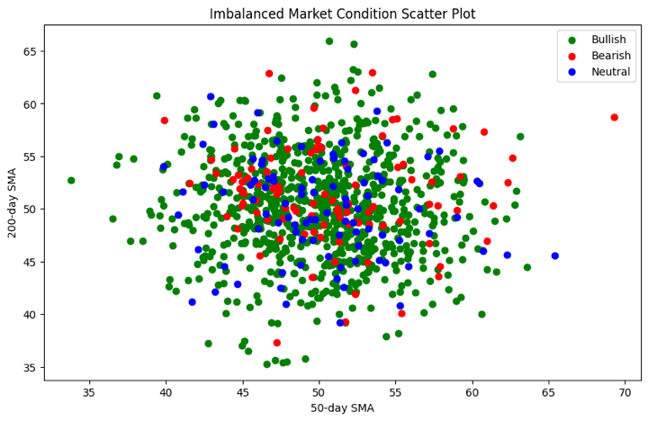
Imbalanced Classification

In imbalanced classification, one class is significantly more prevalent than the others. For example, in fraud detection, the majority of transactions are legitimate, making fraud cases rare. Handling imbalanced datasets is a challenge in such cases.

Let us now see the Python code for learning more about this type.

Output:

Accuracy: 0.81
Classification Report:
              precision    recall  f1-score   support

     Bearish       0.33      0.13      0.19        15
     Bullish       0.82      0.98      0.89       163
     Neutral       0.00      0.00      0.00        22

    accuracy                           0.81       200
   macro avg       0.39      0.37      0.36       200
weighted avg       0.70      0.81      0.74       200

Confusion Matrix:
[[  2  13   0]
 [  3 159   1]
 [  1  21   0]]

Hence, the scatter plot visually demonstrates the class imbalance in the dataset. This way, you can find out which label is making the dataset be imbalanced and thus, base your trading strategy accordingly.

The scatter plot above shows that each market condition (Bullish, Bearish, Neutral) is represented by a different colour. The x-axis represents the 50-day Simple Moving Average (SMA_50), and the y-axis represents the 200-day Simple Moving Average (SMA_200). The mapping of colours is done to visualise the market conditions.

Importance of classification in Machine Learning from trading point of view

From a trading perspective, classification in machine learning holds considerable importance.

Here's why:

• Risk Assessment: Classification models help traders assess and manage risks effectively. By categorising assets or financial instruments based on historical data and market conditions, traders can make informed decisions about when to buy, sell, or hold investments.
• Market Sentiment Analysis: Machine learning classification can be applied to analyse market sentiment. Traders can classify news articles, social media posts, or financial reports as positive, negative, or neutral, providing insights into market sentiment and potential price movements.
  Artificial intelligence in stock trading also helps traders make more informed decisions by analyzing large amounts of data quickly and identifying patterns or trends that humans might miss. This way, AI tools simplify the trading process and enhance a trader's ability to respond to market changes effectively.
• Algorithmic Trading: Classification algorithms play a pivotal role in algorithmic trading strategies. These models can classify market conditions, signals, and trends, allowing automated trading systems to execute orders with precision and speed.
• Portfolio Management: Classification helps traders categorise assets or securities into risk profiles or sectors. This classification aids in constructing well-diversified portfolios that align with an investor's risk tolerance and financial goals.
• Fraud Detection: In trading, particularly in financial markets, fraud detection is critical. Classification models can identify unusual trading patterns or transactions, helping to detect and prevent fraudulent activities.
• Predictive Analytics: Classification models can forecast price movements, market trends, and trading opportunities. By classifying historical data and market indicators, traders can make predictions about future market conditions.
• Trading Strategies: Classification is essential for developing and backtesting trading strategies. Traders can classify data to create rule-based strategies that guide their trading decisions, optimising entry and exit points.
• Risk Management: Accurate classification of trading positions, such as stop-loss orders and profit targets, is vital for risk management. Traders use classification models to set these parameters based on market conditions and historical data.

In summary, classification in machine learning is a cornerstone of trading strategies, aiding traders in risk assessment, market sentiment analysis, algorithmic trading, portfolio management, fraud detection, predictive analytics, strategy development, and risk management. It empowers traders to make data-driven decisions and navigate the complexities of financial markets effectively.

What is the difference between SVM and other classification algorithms?

Following are the key differences between Support Vector Machines (SVM) and other classification algorithms:

It's essential to choose the appropriate classification algorithm based on the specific characteristics of your data and the problem at hand.

SVM excels in scenarios where maximising the margin between classes and handling high-dimensional data are crucial, but it may not always be the best choice for every problem.

Preparing Data for Classification

Preparing data in classification is vital as it ensures that the data is clean, consistent, and suitable for machine learning models. Proper data preprocessing, exploration, and feature engineering enhance model accuracy and performance.

It helps mitigate issues like missing values, outliers, and irrelevant features, enabling models to learn meaningful patterns and make accurate predictions, ultimately leading to more reliable and effective classification outcomes.

For example, in spam email classification, data preparation involves cleaning, extracting relevant features (e.g., content analysis), balancing classes, and text preprocessing (e.g., removing stop words) for accurate classification and reduced false positives.

Here's an overview of the key steps involved in preparing data for classification in machine learning:

Data Collection and Preprocessing

This first step involves the following:

1. Data Collection: Gather relevant data from various sources, ensuring it represents the problem domain accurately. Data sources may include databases, APIs, surveys, or sensor data.
2. Data Cleaning: Identify and handle missing values, duplicates, and outliers to ensure data quality. Impute missing values or remove inconsistent data points.
3. Data Transformation: Convert data types, standardise units, and apply necessary transformations like scaling or log transformations.
4. Encoding Categorical Variables: Convert categorical variables into numerical representations, often using techniques like one-hot encoding or label encoding.

Data Exploration and Visualisation

The second step includes the following:

1. Exploratory Data Analysis (EDA): Explore the dataset to understand its characteristics, distribution, and relationships between variables.
2. Descriptive Statistics: Calculate summary statistics, such as mean, median, and variance, to gain insights into the data's central tendencies and variability.
3. Data Visualisation: Create plots and charts, such as histograms, scatter plots, and box plots, to visualise data patterns, relationships, and anomalies.
4. Correlation Analysis: Examine correlations between features to identify potential multicollinearity or relationships that may affect the model.

Feature Selection and Engineering

The third and the last step is feature selection and engineering. This includes:

1. Feature Selection: Identify the most relevant features that contribute to the classification task. Use techniques like correlation analysis, feature importance scores, or domain knowledge to select important features.
2. Feature Engineering: Create new features or transform existing ones to improve the model's predictive power. This may involve combining, scaling, or extracting meaningful information from features.
3. Dimensionality Reduction: If dealing with high-dimensional data, consider techniques like Principal Component Analysis (PCA) to reduce dimensionality while preserving important information.

By following these steps, you can ensure that your data is well-prepared for classification tasks, which can lead to better model performance and more accurate predictions. Data preprocessing and exploration are critical stages in the machine learning pipeline as they influence the quality of insights and models derived from the data.

Fundamental Concepts

In the realm of machine learning, understanding the fundamental concepts is crucial for building accurate and reliable models. These concepts serve as the building blocks upon which various algorithms and techniques are built.

In this section, we will delve into three essential aspects of machine learning, which are as follows:

1. Supervised Learning Overview
2. Training and Testing Data Split
3. Evaluation Metrics for Classification

Supervised Learning Overview

Supervised learning is a cornerstone of machine learning, where models learn from labelled data to make predictions or classify new, unseen data. In this paradigm, each data point consists of both input features and corresponding target labels. The model learns the relationship between inputs and labels during training and can then generalise its knowledge to make predictions on new, unlabeled data.

Training and Testing Data Split

To assess the performance of a machine learning model, it is essential to split the dataset into two subsets: the training set and the testing set. The training set is used to train the model, allowing it to learn patterns and relationships in the data.

The testing set, which is unseen during training, is used to evaluate how well the model generalises to new data. This split ensures that the model's performance is assessed on data it has not encountered before, helping to gauge its real-world applicability.

Evaluation Metrics for Classification

In classification tasks, the evaluation of model performance is critical. Various metrics are used to assess how well a model classifies data into different classes.

Common metrics include accuracy, precision, recall, F1- score, and the confusion matrix.

• Accuracy measures the overall correctness of predictions, while precision and recall provide insights into a model's ability to correctly classify positive instances.
• The F1-score balances precision and recall.
• The confusion matrix provides a detailed breakdown of true positives, true negatives, false positives, and false negatives.

Understanding these fundamental concepts is essential for practitioners and enthusiasts embarking on their journey into the world of machine learning. They lay the groundwork for effective model development, evaluation, and optimisation, enabling the creation of accurate and reliable predictive systems.

Classification Algorithms

Classification algorithms are a vital component of machine learning, empowering computers to categorise data into distinct classes or groups.

They enable tasks like spam email detection, image recognition, and disease diagnosis by learning from labelled examples to make informed predictions and decisions, making them fundamental tools in various domains.

Let us see a list of classification algorithms below. These classification algorithms are discussed in detail in our learning track Machine learning & Deep learning in trading - 1. These are:

• Linear Models
• Tree-Based Methods
• Support Vector Machines
• Nearest Neighbors
• Naive Bayes
• Neural Networks
• Ensembles

Linear Models

Linear models, like Logistic Regression and Linear Discriminant Analysis, create linear decision boundaries to classify data points. These linear models are a part of quantitative trading. They are simple yet effective for linearly separable data.

For example,

1. In algorithmic trading, Logistic Regression is used to model the likelihood of a stock price movement. It can predict the probability of a stock price increasing or decreasing based on factors like historical price trends, trading volumes, and technical indicators. If the predicted probability exceeds a threshold, a trading decision is made to buy or sell the stock.
2. Traders employ Linear Discriminant Analysis to reduce the dimensionality of their trading data while preserving class separation. LDA can help identify linear combinations of features that maximise the separation between different market conditions, such as bull and bear markets. This reduced-dimensional representation can then be used for decision-making, risk assessment, or portfolio management.

Tree-Based Methods

Tree-based methods, such as Decision trees, Random forest, and Gradient boosting, use hierarchical tree structures to partition data into distinct classes based on feature values.

For example,

1. A trader uses a decision tree to decide whether to buy or sell a particular stock. The decision tree considers factors like historical price trends, trading volumes, and technical indicators to make trading decisions based on predefined rules.
2. In algorithmic trading, a Random Forest model is employed to create an ensemble of decision trees. Each decision tree predicts whether to enter or exit a trade based on different subsets of features. The final trading decision is made by aggregating the predictions of all decision trees in the forest, leading to more robust and accurate trading strategies.
3. Traders use Gradient Boosting to predict stock price movements. Multiple weak predictive models (e.g., decision trees) are iteratively trained to correct the errors of the previous models. This ensemble approach allows for the development of highly accurate trading models capable of capturing complex market dynamics.

Support Vector Machines

SVMs find a hyperplane that maximises the margin between classes, effectively separating data. They work well in both linear and non-linear scenarios.

For example, Separating handwritten digits (such as, 0, 1, 2) in a dataset using SVM to recognise and classify digits in optical character recognition (OCR) systems.

Nearest Neighbors

K-NN classifies data points by considering the majority class among their k-nearest neighbors. It's intuitive and adaptable to various data distributions.

For example, Identifying whether an online review is positive or negative by comparing it to the k-nearest reviews in terms of sentiment and content.

Naive Bayes

Naive Bayes applies Bayes' theorem with the assumption of feature independence. It's efficient for text and categorical data, often used in spam detection and sentiment analysis.

For example, In algorithmic trading, Naive Bayes is used to assess market sentiment from financial news articles. It categorises articles as "Bullish," "Bearish," or "Neutral" based on keyword occurrences, aiding traders' decision-making.

Neural Networks

Neural networks, including feedforward and deep learning models, consist of interconnected artificial neurons. They excel in complex, non-linear tasks like image recognition and natural language processing.

Ensembles

Ensembles combine multiple models to improve classification accuracy. Bagging (e.g., Random Forest), boosting (e.g., AdaBoost), and stacking are ensemble techniques used to enhance predictive power and robustness.

For example, an ensemble of decision trees, like Random Forest, combines the predictions of multiple models to make stock price predictions. It aggregates insights from individual trees to enhance trading strategies.

Challenge: Handling Imbalanced Data

In many real-world scenarios, machine learning datasets suffer from class imbalance, where one class significantly outweighs the others. This creates challenges for models, which may become biassed toward the majority class.

For example, we might have a lot of data on normal market days but very little data on rare events like stock market crashes. This imbalance can make it hard for our trading models to learn and predict accurately.

To address this issue, various techniques and resampling methods are employed to ensure fair and accurate model training and evaluation.

These are as follows:

Techniques for Imbalanced Datasets

Below are a few techniques to handle the imbalanced data.

• Over-sampling: Imagine you have a collection of rare historical market events, like crashes. Over-sampling means creating more copies of these events so that they have as much influence as the more common data in your model. This helps the model understand how to react to rare events better.
• Under-sampling: In this case, you might have too much data on normal market days. Under-sampling means throwing away some of this data to make it more balanced with the rare events. It's like trimming down the common data to focus more on the unusual ones.
• Combined Sampling: Sometimes it's best to use both over-sampling and under-sampling together. This approach balances the dataset by adding more rare events and reducing some of the common ones, giving your model a better perspective.
• Cost-sensitive Learning: Think of this as telling your model that making a mistake with rare events is more costly than making a mistake with common events. It encourages the model to pay extra attention to the rare events, like crashes, when making decisions.

Resampling Methods

Now, let us see the resampling methods below.

• Bootstrap Resampling: Imagine you have a small sample of market data, and you want to understand it better. Bootstrap resampling is like taking small random samples from your small sample many times. This helps you learn more about your data.
• SMOTE (Synthetic Minority Over-sampling Technique): SMOTE is like creating imaginary data points for rare events based on the real data you have. It helps your model understand how to handle rare situations by inventing more examples of them.
• NearMiss: When you have too much data on normal market days, NearMiss is like selecting only a few of them that are closest to the rare events. This way, you keep the most relevant common data and reduce the imbalance.

These methods in trading are like adjusting your telescope's focus to see both the common and rare stars clearly. They help your trading models make better decisions, even in situations that don't happen very often, like major market crashes.

Hyperparameter Tuning or Model optimisation

Hyperparameter tuning, also known as model optimisation, is the process of fine-tuning the settings of a machine learning model to achieve the best performance. These settings, known as hyperparameters, are parameters that are not learned from the data but are set before training the model. In the context of trading, optimising models is essential for creating accurate and successful trading strategies.

For example, Imagine you're trading stocks using a computer language. This computer language has settings that determine how it makes buy and sell decisions, like how much returns you want before selling or how much you're willing to lose before cutting your losses. These settings are called hyperparameters. Hyperparameter tuning is like adjusting these settings to make your trading strategy have maximum returns.

Grid Search

Grid search is like trying out different combinations of settings systematically. Imagine you have a set of parameters to adjust in your trading model (example., the learning rate or the number of trees in a Random Forest).

Grid search helps you create a grid of possible values for each parameter and then tests your model's performance with each combination. It's like exploring a grid to find the best route.

For example, Let's say you're using a trading algorithm that has parameters like the moving average window size and the risk threshold for trades. Grid search helps you test various combinations of these parameters to find the settings that yield the highest returns over historical trading data.

Random Search

Random search is a bit like experimenting with different settings randomly. Instead of testing all possible combinations like in grid search, random search randomly selects values for your model's hyperparameters. It's like trying different keys to unlock a door rather than trying them in a fixed order.

For example, in the trading domain, random search can be applied by randomly selecting values for parameters like stop-loss levels and take-profit thresholds in a trading strategy. It explores a wide range of possibilities to find potentially successful settings.

Bayesian Optimisation

Bayesian optimisation is like having a smart assistant that learns from previous experiments. It uses information from past tests to make informed decisions about which settings to try next. It's like adjusting your trading strategy based on what worked and what didn't in previous trades.

For example, when optimising a trading model, Bayesian optimisation can adaptively select hyperparameter values by considering the historical performance of the strategy. It might adjust the look-back period for a technical indicator based on past trading outcomes, aiming to maximise returns and minimise losses.

Model Evaluation and Selection

In trading, selecting the right machine learning model is crucial for making informed investment decisions. Model evaluation and selection involve assessing the performance of different models and strategies to choose the most effective one.

This process helps traders build robust trading systems and enhance their understanding of market dynamics.

Here are the ways to do model evaluation and selection:

Cross-Validation

Cross-validation is like stress-testing a trading strategy. Instead of using all available data for training, you split it into multiple parts (folds). You train the model on some folds and test it on others, rotating through all folds.

This helps assess how well your strategy performs under various market conditions, ensuring it's not overfitting to a specific time period. In trading, cross-validation ensures your model is adaptable and reliable.

For example, A quantitative trader develops a machine learning-based strategy to predict stock price movements. To ensure the model's robustness, they implement k-fold cross-validation.

They divide historical trading data into, say, 5 folds. They train the model on 4 of these folds and test it on the remaining fold, rotating through all combinations. This helps assess how well the strategy performs across different market conditions, ensuring it's not overfitting to a specific time frame.

Model Selection Strategies

Model selection is like choosing the right tool for the job. In trading, you may consider different models or trading strategies, each with its strengths and weaknesses.

Strategies can be based on technical indicators, sentiment analysis, or fundamental data. You evaluate their historical performance and choose the one that aligns best with your trading goals and risk tolerance. Just like a craftsman selects the right tool, traders select the right strategy for their financial goals.

For example, A portfolio manager wants to choose a trading strategy for a specific market condition—volatility. They consider two strategies: a trend-following approach based on moving averages and a mean-reversion approach using Bollinger Bands.

The manager backtests both strategies over various historical periods of market volatility and selects the one that consistently outperforms in volatile markets, aligning with their risk tolerance and investment goals.

Interpretability and Explainability

Interpretability and explainability are about understanding how and why your trading model makes decisions. Think of it as the user manual for your strategy. In trading, it's crucial to know why the model suggests buying or selling a stock.

This helps traders trust the model and make better-informed decisions. It's like having a clear roadmap to follow in the complex world of financial markets, ensuring your strategies are transparent and accountable.

For example, A hedge fund deploys a machine learning model for stock selection. The model recommends buying certain stocks based on various features. However, the fund's investors and compliance team require transparency.

The fund implements techniques to explain why the model suggests each stock. This involves analysing feature importance, identifying key drivers, and providing clear explanations for each trade recommendation, instilling trust and accountability in the model's decisions.

Using SVC in trading

We will be using Support Vector Machines to implement a simple trading strategy in python. The target variables would be to either buy or sell the stock depending on the feature variables.

We will be using the yahoo finance AAPL dataset to train and test the model. We can download the data using the yfinance library.

You can install the library using the command ‘pip install yfinance’. After installation, load the library and download the dataset.

Output:

Now we must decide the target variable and split the dataset accordingly. For our case, we will use the closing price of the stock to determine whether to buy or sell the stock. If the next trading day's close price is greater than today's close price then, we will buy, else we will sell the stock. We will store +1 for the buy signal and -1 for the sell signal.

X is a dataset that holds the predictor's variables which are used to predict the target variable, ‘y’. X consists of variables such as 'Open - Close' and 'High - Low'. These can be understood as indicators based on which the algorithm will predict the option price.

Now we can split the train and test data and train a simple SVC on this data.

Output:

[*********************100%%**********************]  1 of 1 completed
Accuracy: 0.54
Classification Report:
              precision    recall  f1-score   support

          -1       0.00      0.00      0.00        22
           1       0.54      1.00      0.70        26

    accuracy                           0.54        48
   macro avg       0.27      0.50      0.35        48
weighted avg       0.29      0.54      0.38        48

Now, let us do the evaluation of the machine learning model's performance on the basis of the output above, for the binary classification task.

Let's break it down:

• Accuracy: 0.54: This is the accuracy of the classification model, and it means that the model correctly classified 54% of the total instances. While accuracy is a common metric, it's not always sufficient to evaluate a model's performance, especially when the classes are imbalanced.
• Classification Report: This section provides more detailed information, including precision, recall, and F1-score for each class and some aggregated statistics:
• Precision: It measures the percentage of true positive predictions among all positive predictions. For class -1, the precision is 0.00 (no true positive predictions), and for class 1, it's 0.54, indicating that 54% of the positive predictions for class 1 were correct.
• Recall (Sensitivity): It measures the percentage of true positive predictions among all actual positive instances. For class -1, the recall is 0.00, and for class 1, it's 1.00, indicating that all actual instances of class 1 were correctly predicted.
• F1-Score: It's the harmonic mean of precision and recall, providing a balance between the two metrics. For class -1, the F1-score is 0.00, and for class 1, it's 0.70.
• Support: The number of instances of each class in the dataset.
• Accuracy, macro avg, and weighted avg: These are aggregated statistics:
• Accuracy: We already discussed it; it's the overall accuracy of the model.
• Macro Avg: The average of precision, recall, and F1-score calculated for each class independently and then averaged. In this case, the macro average precision is 0.27, recall is 0.50, and F1-score is 0.35.
• Weighted Avg: Similar to the macro average, but it takes into account the support (the number of instances) for each class. In this case, the weighted average precision is 0.29, recall is 0.54, and F1-score is 0.38.

Overall, this output suggests that the model performs poorly for class -1 but reasonably well for class 1, resulting in a moderate overall accuracy of 0.54. It's important to consider the specific context and requirements of your classification problem to determine whether this level of performance is acceptable.

Additionally, further analysis and potentially model improvement may be needed to address the class imbalance and low performance for class -1.

Resources to learn Machine Learning Classification

• Trading with Machine Learning: Classification and SVM
• Machine Learning Basics
• Scikit Learn Tutorial: Installation, Requirements and Building Classification Model
• Use Decision Trees in Machine Learning to Predict Stock Movements
• Machine Learning Logistic Regression In Python: From Theory To Trading

Conclusion

Machine Learning can be classified into supervised and unsupervised models depending on the presence of target variables. They can also be classified into Regression and Classification models based on the type of target variables.

Various types of classification models include k - nearest neighbors, Support Vector Machines, Decision Trees which can be improved by using Ensemble Learning. This leads to Random Forest Classifiers which are made up of an ensemble of decision trees that learn from each other to improve model accuracy.

You can also improve model accuracy by using hyperparameter tuning techniques such as GridSearchCV and k - fold Cross-Validation. We can test the accuracy of the models by using evaluation methods such as Confusion Matrices, finding a good Precision-Recall tradeoff and using the Area under the ROC curve. We have also looked at how we can use SVC for use in trading strategies.

If you wish to explore more about machine learning classification, you must explore our course on Trading with classification and SVM. With this course, you will learn to use SVM on financial markets data and create your own prediction algorithm. The course covers classification algorithms, performance measures in machine learning, hyper-parameters and building of supervised classifiers.

Note: The original post has been revamped on 30th November 2023 for accuracy, and recentness.

Disclaimer: All data and information provided in this article are for informational purposes only. QuantInsti^® makes no representations as to accuracy, completeness, currentness, suitability, or validity of any information in this article and will not be liable for any errors, omissions, or delays in this information or any losses, injuries, or damages arising from its display or use. All information is provided on an as-is basis.